知识蒸馏教程

创建于： Aug 22, 2023 | 最后更新于： Jan 24, 2025 | 最后验证于： Nov 05, 2024

作者: Alexandros Chariton

知识蒸馏是一种技术，它能够在不损失有效性的前提下，将知识从大型、计算开销大的模型转移到小型模型。这使得模型能够部署在算力较低的硬件上，评估更快且更高效。

在本教程中，我们将进行一系列实验，旨在通过使用更强大的网络作为教师网络，来提高轻量级神经网络的准确性。轻量级网络的计算开销和速度不会受到影响，我们的干预只集中在其权重上，而非其前向传播过程。这项技术的应用可以在无人机或手机等设备中找到。在本教程中，我们不使用任何外部包，因为所需的一切都可以在 torch 和 torchvision 中获得。

在本教程中，您将学习

• 如何修改模型类以提取隐藏表示并将其用于进一步计算

• 如何修改 PyTorch 中的常规训练循环，在例如用于分类任务的交叉熵损失之上，包含额外的损失函数

• 如何通过使用更复杂的模型作为教师网络来提高轻量级模型的性能

前提条件

• 1 个 GPU，4GB 显存

• PyTorch v2.0 或更高版本

• CIFAR-10 数据集（由脚本下载并保存在名为 /data 的目录中）

import torch
import torch.nn as nn
import torch.optim as optim
import torchvision.transforms as transforms
import torchvision.datasets as datasets

# Check if the current `accelerator <https://pytorch.ac.cn/docs/stable/torch.html#accelerators>`__
# is available, and if not, use the CPU
device = torch.accelerator.current_accelerator().type if torch.accelerator.is_available() else "cpu"
print(f"Using {device} device")

Using cuda device

加载 CIFAR-10

CIFAR-10 是一个流行的图像数据集，包含十个类别。我们的目标是为每个输入图像预测以下类别之一。

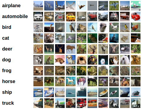
CIFAR-10 图像示例

输入图像是 RGB 格式，因此它们有 3 个通道，大小为 32x32 像素。基本上，每个图像由 3 x 32 x 32 = 3072 个介于 0 到 255 之间的数字描述。神经网络中的常见做法是归一化输入，这样做有多种原因，包括避免常用激活函数饱和以及提高数值稳定性。我们的归一化过程包括减去每个通道的均值并除以标准差。张量“mean=[0.485, 0.456, 0.406]”和“std=[0.229, 0.224, 0.225]”已被计算出来，它们代表了 CIFAR-10 中预定义训练集的每个通道的均值和标准差。注意，我们在测试集上也使用了这些值，而没有从头重新计算均值和标准差。这是因为网络是基于减去和除以上述数字后产生的特征进行训练的，我们希望保持一致性。此外，在实际应用中，我们将无法计算测试集的均值和标准差，因为根据我们的假设，那时这些数据将无法访问。

最后一点，我们通常将这个保留集称为验证集，在优化模型在验证集上的性能后，我们使用一个单独的集合，称为测试集。这样做是为了避免基于对单一指标的贪婪和有偏优化来选择模型。

# Below we are preprocessing data for CIFAR-10. We use an arbitrary batch size of 128.
transforms_cifar = transforms.Compose([
    transforms.ToTensor(),
    transforms.Normalize(mean=[0.485, 0.456, 0.406], std=[0.229, 0.224, 0.225]),
])

# Loading the CIFAR-10 dataset:
train_dataset = datasets.CIFAR10(root='./data', train=True, download=True, transform=transforms_cifar)
test_dataset = datasets.CIFAR10(root='./data', train=False, download=True, transform=transforms_cifar)

  0%|          | 0.00/170M [00:00<?, ?B/s]
  0%|          | 426k/170M [00:00<00:41, 4.10MB/s]
  3%|2         | 4.85M/170M [00:00<00:06, 27.2MB/s]
  6%|5         | 9.67M/170M [00:00<00:04, 36.6MB/s]
  8%|8         | 13.9M/170M [00:00<00:04, 38.6MB/s]
 10%|#         | 17.8M/170M [00:00<00:04, 33.1MB/s]
 12%|#2        | 21.2M/170M [00:00<00:04, 30.1MB/s]
 14%|#4        | 24.4M/170M [00:00<00:05, 28.6MB/s]
 16%|#6        | 27.3M/170M [00:00<00:05, 27.3MB/s]
 18%|#7        | 30.1M/170M [00:01<00:05, 26.7MB/s]
 19%|#9        | 32.8M/170M [00:01<00:05, 26.6MB/s]
 21%|##        | 35.5M/170M [00:01<00:05, 26.4MB/s]
 22%|##2       | 38.2M/170M [00:01<00:05, 26.1MB/s]
 24%|##4       | 41.0M/170M [00:01<00:04, 26.6MB/s]
 26%|##6       | 44.6M/170M [00:01<00:04, 29.2MB/s]
 28%|##8       | 47.9M/170M [00:01<00:04, 30.2MB/s]
 30%|###       | 51.4M/170M [00:01<00:03, 31.5MB/s]
 32%|###2      | 54.8M/170M [00:01<00:03, 31.9MB/s]
 34%|###4      | 58.2M/170M [00:01<00:03, 32.5MB/s]
 36%|###6      | 61.5M/170M [00:02<00:03, 32.6MB/s]
 38%|###8      | 64.8M/170M [00:02<00:03, 32.6MB/s]
 40%|###9      | 68.1M/170M [00:02<00:03, 32.3MB/s]
 42%|####1     | 71.3M/170M [00:02<00:03, 32.0MB/s]
 44%|####3     | 74.5M/170M [00:02<00:03, 31.7MB/s]
 46%|####5     | 77.7M/170M [00:02<00:03, 30.2MB/s]
 47%|####7     | 80.8M/170M [00:02<00:03, 27.3MB/s]
 49%|####9     | 83.6M/170M [00:02<00:03, 25.6MB/s]
 51%|#####     | 86.2M/170M [00:02<00:03, 24.4MB/s]
 52%|#####2    | 88.7M/170M [00:03<00:03, 23.8MB/s]
 53%|#####3    | 91.1M/170M [00:03<00:03, 23.3MB/s]
 55%|#####4    | 93.5M/170M [00:03<00:03, 22.9MB/s]
 56%|#####6    | 95.8M/170M [00:03<00:03, 22.7MB/s]
 58%|#####7    | 98.1M/170M [00:03<00:03, 22.4MB/s]
 59%|#####8    | 100M/170M [00:03<00:03, 22.3MB/s]
 60%|######    | 103M/170M [00:03<00:03, 22.2MB/s]
 61%|######1   | 105M/170M [00:03<00:02, 22.1MB/s]
 63%|######2   | 107M/170M [00:03<00:02, 21.9MB/s]
 64%|######4   | 109M/170M [00:04<00:02, 22.1MB/s]
 65%|######5   | 112M/170M [00:04<00:02, 21.9MB/s]
 67%|######6   | 114M/170M [00:04<00:02, 21.8MB/s]
 68%|######8   | 116M/170M [00:04<00:02, 21.9MB/s]
 69%|######9   | 118M/170M [00:04<00:02, 21.8MB/s]
 71%|#######   | 120M/170M [00:04<00:02, 21.9MB/s]
 72%|#######1  | 123M/170M [00:04<00:02, 21.8MB/s]
 73%|#######3  | 125M/170M [00:04<00:02, 21.8MB/s]
 75%|#######4  | 127M/170M [00:04<00:01, 21.8MB/s]
 76%|#######5  | 129M/170M [00:04<00:01, 21.8MB/s]
 77%|#######7  | 131M/170M [00:05<00:01, 21.5MB/s]
 78%|#######8  | 134M/170M [00:05<00:01, 21.4MB/s]
 80%|#######9  | 136M/170M [00:05<00:01, 21.5MB/s]
 81%|########  | 138M/170M [00:05<00:01, 21.2MB/s]
 82%|########2 | 140M/170M [00:05<00:01, 21.1MB/s]
 83%|########3 | 142M/170M [00:05<00:01, 20.9MB/s]
 85%|########4 | 144M/170M [00:05<00:01, 21.2MB/s]
 86%|########5 | 147M/170M [00:05<00:01, 21.1MB/s]
 87%|########7 | 149M/170M [00:05<00:01, 20.1MB/s]
 88%|########8 | 151M/170M [00:06<00:01, 19.0MB/s]
 90%|########9 | 153M/170M [00:06<00:00, 18.9MB/s]
 91%|######### | 155M/170M [00:06<00:00, 19.3MB/s]
 92%|#########1| 157M/170M [00:06<00:00, 18.8MB/s]
 93%|#########3| 159M/170M [00:06<00:00, 18.8MB/s]
 94%|#########4| 160M/170M [00:06<00:00, 17.7MB/s]
 95%|#########5| 162M/170M [00:06<00:00, 16.3MB/s]
 96%|#########6| 164M/170M [00:06<00:00, 15.3MB/s]
 97%|#########7| 166M/170M [00:06<00:00, 14.8MB/s]
 98%|#########7| 167M/170M [00:07<00:00, 14.4MB/s]
 99%|#########8| 169M/170M [00:07<00:00, 14.1MB/s]
100%|#########9| 170M/170M [00:07<00:00, 13.8MB/s]
100%|##########| 170M/170M [00:07<00:00, 23.3MB/s]

注意

本节仅适用于对快速获得结果感兴趣的 CPU 用户。仅当您对小规模实验感兴趣时使用此选项。请记住，使用任何 GPU 代码都应该运行得相当快。仅从训练/测试数据集中选择前 num_images_to_keep 个图像

#from torch.utils.data import Subset
#num_images_to_keep = 2000
#train_dataset = Subset(train_dataset, range(min(num_images_to_keep, 50_000)))
#test_dataset = Subset(test_dataset, range(min(num_images_to_keep, 10_000)))

#Dataloaders
train_loader = torch.utils.data.DataLoader(train_dataset, batch_size=128, shuffle=True, num_workers=2)
test_loader = torch.utils.data.DataLoader(test_dataset, batch_size=128, shuffle=False, num_workers=2)

定义模型类和辅助函数

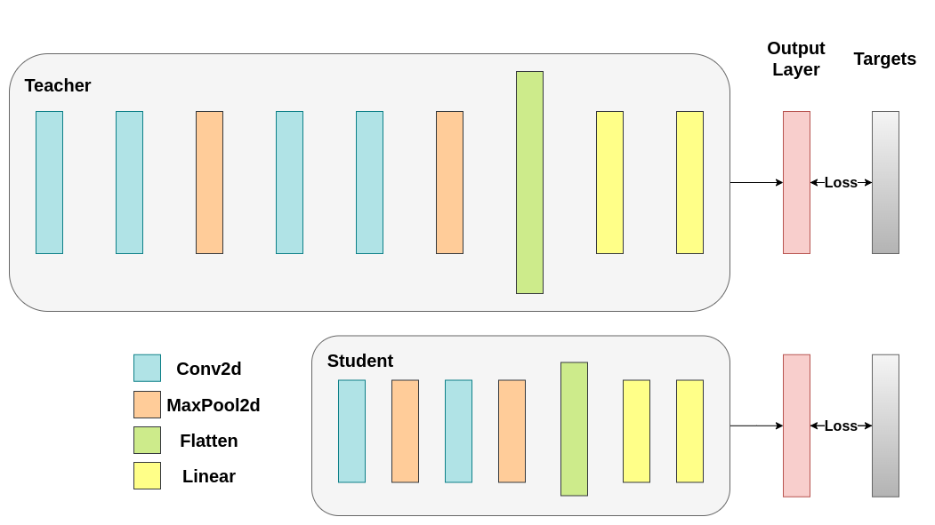
接下来，我们需要定义我们的模型类。这里需要设置几个用户定义参数。我们使用两种不同的架构，在实验中保持滤波器数量固定，以确保公平比较。两种架构都是卷积神经网络 (CNN)，具有不同数量的卷积层作为特征提取器，后跟一个具有 10 个类别的分类器。学生网络的滤波器和神经元数量较少。

# Deeper neural network class to be used as teacher:
class DeepNN(nn.Module):
    def __init__(self, num_classes=10):
        super(DeepNN, self).__init__()
        self.features = nn.Sequential(
            nn.Conv2d(3, 128, kernel_size=3, padding=1),
            nn.ReLU(),
            nn.Conv2d(128, 64, kernel_size=3, padding=1),
            nn.ReLU(),
            nn.MaxPool2d(kernel_size=2, stride=2),
            nn.Conv2d(64, 64, kernel_size=3, padding=1),
            nn.ReLU(),
            nn.Conv2d(64, 32, kernel_size=3, padding=1),
            nn.ReLU(),
            nn.MaxPool2d(kernel_size=2, stride=2),
        )
        self.classifier = nn.Sequential(
            nn.Linear(2048, 512),
            nn.ReLU(),
            nn.Dropout(0.1),
            nn.Linear(512, num_classes)
        )

    def forward(self, x):
        x = self.features(x)
        x = torch.flatten(x, 1)
        x = self.classifier(x)
        return x

# Lightweight neural network class to be used as student:
class LightNN(nn.Module):
    def __init__(self, num_classes=10):
        super(LightNN, self).__init__()
        self.features = nn.Sequential(
            nn.Conv2d(3, 16, kernel_size=3, padding=1),
            nn.ReLU(),
            nn.MaxPool2d(kernel_size=2, stride=2),
            nn.Conv2d(16, 16, kernel_size=3, padding=1),
            nn.ReLU(),
            nn.MaxPool2d(kernel_size=2, stride=2),
        )
        self.classifier = nn.Sequential(
            nn.Linear(1024, 256),
            nn.ReLU(),
            nn.Dropout(0.1),
            nn.Linear(256, num_classes)
        )

    def forward(self, x):
        x = self.features(x)
        x = torch.flatten(x, 1)
        x = self.classifier(x)
        return x

我们使用 2 个函数来帮助我们在原始分类任务上产生和评估结果。其中一个函数称为 train，接受以下参数

• model: 通过此函数训练（更新权重）的模型实例。

• train_loader: 我们在上面定义了 train_loader，它的作用是将数据馈送到模型。

• epochs: 我们遍历数据集的次数。

• learning_rate: 学习率决定了我们朝着收敛方向迈进的步长。步长过大或过小都可能有害。

• device: 确定运行工作负载的设备。可以是 CPU 或 GPU，取决于可用性。

我们的测试函数类似，但会使用 test_loader 来加载测试集中的图像。

使用交叉熵训练两个网络。学生网络将用作基线：

def train(model, train_loader, epochs, learning_rate, device):
    criterion = nn.CrossEntropyLoss()
    optimizer = optim.Adam(model.parameters(), lr=learning_rate)

    model.train()

    for epoch in range(epochs):
        running_loss = 0.0
        for inputs, labels in train_loader:
            # inputs: A collection of batch_size images
            # labels: A vector of dimensionality batch_size with integers denoting class of each image
            inputs, labels = inputs.to(device), labels.to(device)

            optimizer.zero_grad()
            outputs = model(inputs)

            # outputs: Output of the network for the collection of images. A tensor of dimensionality batch_size x num_classes
            # labels: The actual labels of the images. Vector of dimensionality batch_size
            loss = criterion(outputs, labels)
            loss.backward()
            optimizer.step()

            running_loss += loss.item()

        print(f"Epoch {epoch+1}/{epochs}, Loss: {running_loss / len(train_loader)}")

def test(model, test_loader, device):
    model.to(device)
    model.eval()

    correct = 0
    total = 0

    with torch.no_grad():
        for inputs, labels in test_loader:
            inputs, labels = inputs.to(device), labels.to(device)

            outputs = model(inputs)
            _, predicted = torch.max(outputs.data, 1)

            total += labels.size(0)
            correct += (predicted == labels).sum().item()

    accuracy = 100 * correct / total
    print(f"Test Accuracy: {accuracy:.2f}%")
    return accuracy

交叉熵运行

为了可重复性，我们需要设置 torch 手动种子。我们使用不同的方法训练网络，因此为了公平比较，最好用相同的权重初始化网络。首先使用交叉熵训练教师网络

torch.manual_seed(42)
nn_deep = DeepNN(num_classes=10).to(device)
train(nn_deep, train_loader, epochs=10, learning_rate=0.001, device=device)
test_accuracy_deep = test(nn_deep, test_loader, device)

# Instantiate the lightweight network:
torch.manual_seed(42)
nn_light = LightNN(num_classes=10).to(device)

Epoch 1/10, Loss: 1.348291786125554
Epoch 2/10, Loss: 0.8802619594747149
Epoch 3/10, Loss: 0.6910638084344547
Epoch 4/10, Loss: 0.5453190243305148
Epoch 5/10, Loss: 0.4225382124600203
Epoch 6/10, Loss: 0.3179327983151921
Epoch 7/10, Loss: 0.22859162307532546
Epoch 8/10, Loss: 0.16856732934027377
Epoch 9/10, Loss: 0.14358678597318547
Epoch 10/10, Loss: 0.12967746109818407
Test Accuracy: 75.62%

我们再实例化一个轻量级网络模型来比较它们的性能。反向传播对权重初始化很敏感，因此我们需要确保这两个网络具有完全相同的初始化。

torch.manual_seed(42)
new_nn_light = LightNN(num_classes=10).to(device)

为了确保我们创建了第一个网络的副本，我们检查其第一层的范数。如果匹配，我们可以放心地得出结论，这两个网络确实是相同的。

# Print the norm of the first layer of the initial lightweight model
print("Norm of 1st layer of nn_light:", torch.norm(nn_light.features[0].weight).item())
# Print the norm of the first layer of the new lightweight model
print("Norm of 1st layer of new_nn_light:", torch.norm(new_nn_light.features[0].weight).item())

Norm of 1st layer of nn_light: 2.327361822128296
Norm of 1st layer of new_nn_light: 2.327361822128296

打印每个模型中的总参数数量

total_params_deep = "{:,}".format(sum(p.numel() for p in nn_deep.parameters()))
print(f"DeepNN parameters: {total_params_deep}")
total_params_light = "{:,}".format(sum(p.numel() for p in nn_light.parameters()))
print(f"LightNN parameters: {total_params_light}")

DeepNN parameters: 1,186,986
LightNN parameters: 267,738

使用交叉熵损失训练并测试轻量级网络

train(nn_light, train_loader, epochs=10, learning_rate=0.001, device=device)
test_accuracy_light_ce = test(nn_light, test_loader, device)

Epoch 1/10, Loss: 1.4697812533439578
Epoch 2/10, Loss: 1.153727483871343
Epoch 3/10, Loss: 1.0198465607050435
Epoch 4/10, Loss: 0.9203303406000747
Epoch 5/10, Loss: 0.8472354605679622
Epoch 6/10, Loss: 0.7809330093891115
Epoch 7/10, Loss: 0.7178317027171249
Epoch 8/10, Loss: 0.660715803084776
Epoch 9/10, Loss: 0.6083721332537854
Epoch 10/10, Loss: 0.5571968615664851
Test Accuracy: 70.43%

正如我们所见，基于测试准确性，我们现在可以将用作教师网络的更深层网络与我们预期的学生网络进行比较。到目前为止，学生网络尚未与教师网络进行干预，因此这个性能是学生网络本身实现的。当前的指标可以通过以下行看到

print(f"Teacher accuracy: {test_accuracy_deep:.2f}%")
print(f"Student accuracy: {test_accuracy_light_ce:.2f}%")

Teacher accuracy: 75.62%
Student accuracy: 70.43%

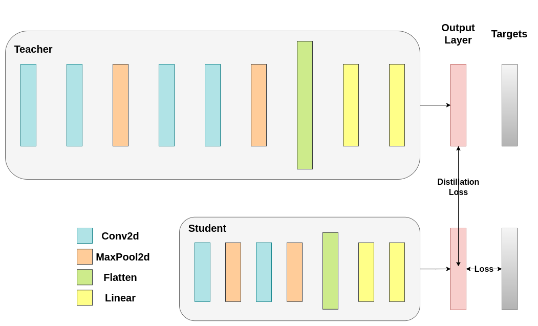
知识蒸馏运行

现在，让我们尝试通过融入教师网络来提高学生网络的测试准确性。知识蒸馏是一种直接的技术，其基础是两个网络都输出关于类别的概率分布。因此，两个网络共享相同数量的输出神经元。该方法通过在传统的交叉熵损失中加入一个额外的损失来实现，这个额外的损失基于教师网络的 softmax 输出。其假设是，经过适当训练的教师网络的输出激活携带了学生网络在训练期间可以利用的额外信息。原始研究表明，利用软目标中较小概率的比率有助于实现深度神经网络的潜在目标，即在数据上创建一种相似性结构，将相似的对象映射得更近。例如，在 CIFAR-10 中，一辆卡车如果存在轮子，可能会被误认为是汽车或飞机，但不太可能被误认为是狗。因此，可以合理地假设有价值的信息不仅存在于经过适当训练的模型的最高预测中，还存在于整个输出分布中。然而，仅凭交叉熵无法充分利用这些信息，因为非预测类别的激活往往非常小，导致传播的梯度无法有效地改变权重来构建这种理想的向量空间。

当我们继续定义引入教师-学生动态的第一个辅助函数时，需要包含一些额外的参数

• T: 温度，控制输出分布的平滑度。较大的 T 会导致更平滑的分布，从而使较小的概率获得更大的提升。

• soft_target_loss_weight: 分配给我们即将包含的额外目标的权重。

• ce_loss_weight: 分配给交叉熵的权重。调整这些权重会使网络倾向于优化其中任一目标。

蒸馏损失是根据网络的 logits 计算的。它只向学生网络返回梯度：

def train_knowledge_distillation(teacher, student, train_loader, epochs, learning_rate, T, soft_target_loss_weight, ce_loss_weight, device):
    ce_loss = nn.CrossEntropyLoss()
    optimizer = optim.Adam(student.parameters(), lr=learning_rate)

    teacher.eval()  # Teacher set to evaluation mode
    student.train() # Student to train mode

    for epoch in range(epochs):
        running_loss = 0.0
        for inputs, labels in train_loader:
            inputs, labels = inputs.to(device), labels.to(device)

            optimizer.zero_grad()

            # Forward pass with the teacher model - do not save gradients here as we do not change the teacher's weights
            with torch.no_grad():
                teacher_logits = teacher(inputs)

            # Forward pass with the student model
            student_logits = student(inputs)

            #Soften the student logits by applying softmax first and log() second
            soft_targets = nn.functional.softmax(teacher_logits / T, dim=-1)
            soft_prob = nn.functional.log_softmax(student_logits / T, dim=-1)

            # Calculate the soft targets loss. Scaled by T**2 as suggested by the authors of the paper "Distilling the knowledge in a neural network"
            soft_targets_loss = torch.sum(soft_targets * (soft_targets.log() - soft_prob)) / soft_prob.size()[0] * (T**2)

            # Calculate the true label loss
            label_loss = ce_loss(student_logits, labels)

            # Weighted sum of the two losses
            loss = soft_target_loss_weight * soft_targets_loss + ce_loss_weight * label_loss

            loss.backward()
            optimizer.step()

            running_loss += loss.item()

        print(f"Epoch {epoch+1}/{epochs}, Loss: {running_loss / len(train_loader)}")

# Apply ``train_knowledge_distillation`` with a temperature of 2. Arbitrarily set the weights to 0.75 for CE and 0.25 for distillation loss.
train_knowledge_distillation(teacher=nn_deep, student=new_nn_light, train_loader=train_loader, epochs=10, learning_rate=0.001, T=2, soft_target_loss_weight=0.25, ce_loss_weight=0.75, device=device)
test_accuracy_light_ce_and_kd = test(new_nn_light, test_loader, device)

# Compare the student test accuracy with and without the teacher, after distillation
print(f"Teacher accuracy: {test_accuracy_deep:.2f}%")
print(f"Student accuracy without teacher: {test_accuracy_light_ce:.2f}%")
print(f"Student accuracy with CE + KD: {test_accuracy_light_ce_and_kd:.2f}%")

Epoch 1/10, Loss: 2.386750131921695
Epoch 2/10, Loss: 1.868185037237299
Epoch 3/10, Loss: 1.642685822513707
Epoch 4/10, Loss: 1.484524897602208
Epoch 5/10, Loss: 1.3599990208435546
Epoch 6/10, Loss: 1.2424575910543847
Epoch 7/10, Loss: 1.147350205942188
Epoch 8/10, Loss: 1.0649026226814446
Epoch 9/10, Loss: 0.9886922711301642
Epoch 10/10, Loss: 0.9178902323898452
Test Accuracy: 70.48%
Teacher accuracy: 75.62%
Student accuracy without teacher: 70.43%
Student accuracy with CE + KD: 70.48%

余弦损失最小化运行

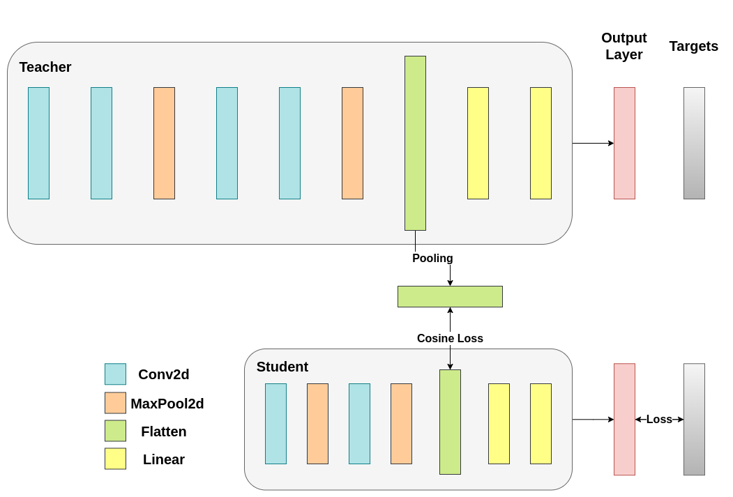
您可以随意调整控制 softmax 函数软化程度的温度参数和损失系数。在神经网络中，很容易为主目标添加额外的损失函数，以实现更好的泛化等目标。让我们尝试为学生网络包含一个目标，但现在我们将重点放在它们的隐藏状态，而不是输出层。我们的目标是通过包含一个朴素的损失函数，将信息从教师网络的表示传递给学生网络。这个损失函数的最小化意味着随后传递给分类器的扁平化向量随着损失的减小变得更相似。当然，教师网络不会更新其权重，因此最小化仅取决于学生网络的权重。这种方法背后的原理是，我们假设教师模型具有更好的内部表示，学生网络在没有外部干预的情况下不太可能达到这种表示，因此我们人工地推动学生网络模仿教师网络的内部表示。然而，这是否最终会帮助学生网络并不简单，因为将轻量级网络推向这个点可能是一件好事，前提是我们找到了一个能带来更好测试准确性的内部表示，但也可能有害，因为网络具有不同的架构，学生网络没有与教师网络相同的学习能力。换句话说，学生和教师的这两个向量没有理由在每个组件上完全匹配。学生网络可以达到一个内部表示，它是教师网络表示的一个排列，并且效率相同。尽管如此，我们仍然可以进行一个快速实验来弄清楚这种方法的影响。我们将使用 CosineEmbeddingLoss，它的公式如下

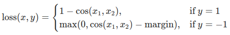
CosineEmbeddingLoss 公式

显然，我们首先需要解决一个问题。当我们对输出层应用蒸馏时，我们提到两个网络都具有相同数量的神经元，等于类别的数量。然而，对于卷积层之后的层来说并非如此。在这里，在最终卷积层展平后，教师网络比学生网络拥有更多神经元。我们的损失函数接受两个维度相同的向量作为输入，因此我们需要以某种方式匹配它们。我们将通过在教师网络的卷积层之后包含一个平均池化层来解决这个问题，以减小其维度，使其与学生网络的维度匹配。

为了继续，我们将修改我们的模型类，或创建新的模型类。现在，前向传播函数不仅返回网络的 logits，还返回卷积层之后的展平隐藏表示。我们为修改后的教师网络包含了上述池化层。

class ModifiedDeepNNCosine(nn.Module):
    def __init__(self, num_classes=10):
        super(ModifiedDeepNNCosine, self).__init__()
        self.features = nn.Sequential(
            nn.Conv2d(3, 128, kernel_size=3, padding=1),
            nn.ReLU(),
            nn.Conv2d(128, 64, kernel_size=3, padding=1),
            nn.ReLU(),
            nn.MaxPool2d(kernel_size=2, stride=2),
            nn.Conv2d(64, 64, kernel_size=3, padding=1),
            nn.ReLU(),
            nn.Conv2d(64, 32, kernel_size=3, padding=1),
            nn.ReLU(),
            nn.MaxPool2d(kernel_size=2, stride=2),
        )
        self.classifier = nn.Sequential(
            nn.Linear(2048, 512),
            nn.ReLU(),
            nn.Dropout(0.1),
            nn.Linear(512, num_classes)
        )

    def forward(self, x):
        x = self.features(x)
        flattened_conv_output = torch.flatten(x, 1)
        x = self.classifier(flattened_conv_output)
        flattened_conv_output_after_pooling = torch.nn.functional.avg_pool1d(flattened_conv_output, 2)
        return x, flattened_conv_output_after_pooling

# Create a similar student class where we return a tuple. We do not apply pooling after flattening.
class ModifiedLightNNCosine(nn.Module):
    def __init__(self, num_classes=10):
        super(ModifiedLightNNCosine, self).__init__()
        self.features = nn.Sequential(
            nn.Conv2d(3, 16, kernel_size=3, padding=1),
            nn.ReLU(),
            nn.MaxPool2d(kernel_size=2, stride=2),
            nn.Conv2d(16, 16, kernel_size=3, padding=1),
            nn.ReLU(),
            nn.MaxPool2d(kernel_size=2, stride=2),
        )
        self.classifier = nn.Sequential(
            nn.Linear(1024, 256),
            nn.ReLU(),
            nn.Dropout(0.1),
            nn.Linear(256, num_classes)
        )

    def forward(self, x):
        x = self.features(x)
        flattened_conv_output = torch.flatten(x, 1)
        x = self.classifier(flattened_conv_output)
        return x, flattened_conv_output

# We do not have to train the modified deep network from scratch of course, we just load its weights from the trained instance
modified_nn_deep = ModifiedDeepNNCosine(num_classes=10).to(device)
modified_nn_deep.load_state_dict(nn_deep.state_dict())

# Once again ensure the norm of the first layer is the same for both networks
print("Norm of 1st layer for deep_nn:", torch.norm(nn_deep.features[0].weight).item())
print("Norm of 1st layer for modified_deep_nn:", torch.norm(modified_nn_deep.features[0].weight).item())

# Initialize a modified lightweight network with the same seed as our other lightweight instances. This will be trained from scratch to examine the effectiveness of cosine loss minimization.
torch.manual_seed(42)
modified_nn_light = ModifiedLightNNCosine(num_classes=10).to(device)
print("Norm of 1st layer:", torch.norm(modified_nn_light.features[0].weight).item())

Norm of 1st layer for deep_nn: 7.503714084625244
Norm of 1st layer for modified_deep_nn: 7.503714084625244
Norm of 1st layer: 2.327361822128296

自然地，我们需要更改训练循环，因为现在模型返回一个元组 (logits, hidden_representation)。使用一个示例输入张量，我们可以打印它们的形状。

# Create a sample input tensor
sample_input = torch.randn(128, 3, 32, 32).to(device) # Batch size: 128, Filters: 3, Image size: 32x32

# Pass the input through the student
logits, hidden_representation = modified_nn_light(sample_input)

# Print the shapes of the tensors
print("Student logits shape:", logits.shape) # batch_size x total_classes
print("Student hidden representation shape:", hidden_representation.shape) # batch_size x hidden_representation_size

# Pass the input through the teacher
logits, hidden_representation = modified_nn_deep(sample_input)

# Print the shapes of the tensors
print("Teacher logits shape:", logits.shape) # batch_size x total_classes
print("Teacher hidden representation shape:", hidden_representation.shape) # batch_size x hidden_representation_size

Student logits shape: torch.Size([128, 10])
Student hidden representation shape: torch.Size([128, 1024])
Teacher logits shape: torch.Size([128, 10])
Teacher hidden representation shape: torch.Size([128, 1024])

在我们的例子中，hidden_representation_size 是 1024。这是学生网络最终卷积层的展平特征图，如您所见，它是其分类器的输入。对于教师网络也是 1024，因为我们使用 avg_pool1d 将其从 2048 变为了 1024。这里应用的损失仅影响学生网络在损失计算之前的权重。换句话说，它不影响学生网络的分类器。修改后的训练循环如下

在余弦损失最小化中，我们希望通过向学生网络返回梯度来最大化两个表示的余弦相似度：

def train_cosine_loss(teacher, student, train_loader, epochs, learning_rate, hidden_rep_loss_weight, ce_loss_weight, device):
    ce_loss = nn.CrossEntropyLoss()
    cosine_loss = nn.CosineEmbeddingLoss()
    optimizer = optim.Adam(student.parameters(), lr=learning_rate)

    teacher.to(device)
    student.to(device)
    teacher.eval()  # Teacher set to evaluation mode
    student.train() # Student to train mode

    for epoch in range(epochs):
        running_loss = 0.0
        for inputs, labels in train_loader:
            inputs, labels = inputs.to(device), labels.to(device)

            optimizer.zero_grad()

            # Forward pass with the teacher model and keep only the hidden representation
            with torch.no_grad():
                _, teacher_hidden_representation = teacher(inputs)

            # Forward pass with the student model
            student_logits, student_hidden_representation = student(inputs)

            # Calculate the cosine loss. Target is a vector of ones. From the loss formula above we can see that is the case where loss minimization leads to cosine similarity increase.
            hidden_rep_loss = cosine_loss(student_hidden_representation, teacher_hidden_representation, target=torch.ones(inputs.size(0)).to(device))

            # Calculate the true label loss
            label_loss = ce_loss(student_logits, labels)

            # Weighted sum of the two losses
            loss = hidden_rep_loss_weight * hidden_rep_loss + ce_loss_weight * label_loss

            loss.backward()
            optimizer.step()

            running_loss += loss.item()

        print(f"Epoch {epoch+1}/{epochs}, Loss: {running_loss / len(train_loader)}")

由于同样的原因，我们需要修改我们的测试函数。在这里，我们忽略了模型返回的隐藏表示。

def test_multiple_outputs(model, test_loader, device):
    model.to(device)
    model.eval()

    correct = 0
    total = 0

    with torch.no_grad():
        for inputs, labels in test_loader:
            inputs, labels = inputs.to(device), labels.to(device)

            outputs, _ = model(inputs) # Disregard the second tensor of the tuple
            _, predicted = torch.max(outputs.data, 1)

            total += labels.size(0)
            correct += (predicted == labels).sum().item()

    accuracy = 100 * correct / total
    print(f"Test Accuracy: {accuracy:.2f}%")
    return accuracy

在这种情况下，我们可以很容易地将知识蒸馏和余弦损失最小化包含在同一个函数中。在教师-学生范式中，结合多种方法来获得更好的性能是常见的。现在，我们可以运行一个简单的训练-测试会话。

# Train and test the lightweight network with cross entropy loss
train_cosine_loss(teacher=modified_nn_deep, student=modified_nn_light, train_loader=train_loader, epochs=10, learning_rate=0.001, hidden_rep_loss_weight=0.25, ce_loss_weight=0.75, device=device)
test_accuracy_light_ce_and_cosine_loss = test_multiple_outputs(modified_nn_light, test_loader, device)

Epoch 1/10, Loss: 1.3048658852686967
Epoch 2/10, Loss: 1.0663291737246696
Epoch 3/10, Loss: 0.9672873822014655
Epoch 4/10, Loss: 0.8923313494228646
Epoch 5/10, Loss: 0.8383791920779001
Epoch 6/10, Loss: 0.7914473272650443
Epoch 7/10, Loss: 0.7511683412829934
Epoch 8/10, Loss: 0.7156466943833529
Epoch 9/10, Loss: 0.6772932203681877
Epoch 10/10, Loss: 0.6502810129729073
Test Accuracy: 70.76%

中间回归器运行

我们朴素的最小化方法并不能保证更好的结果，原因有几个，其中之一是向量的维度。对于高维向量，余弦相似度通常比欧几里得距离效果更好，但我们处理的是每个向量有 1024 个分量，因此更难提取有意义的相似性。此外，正如我们所提到的，理论上并不支持推动教师网络和学生网络的隐藏表示完全匹配。没有充分的理由说明我们应该追求这些向量的 1:1 匹配。我们将提供最后一个训练干预的例子，即包含一个额外的网络，称为回归器（regressor）。目标是首先提取教师网络在卷积层后的特征图，然后提取学生网络在卷积层后的特征图，最后尝试匹配这些特征图。然而，这一次，我们将在网络之间引入一个回归器来促进匹配过程。回归器将是可训练的，并且理想情况下会比我们朴素的余弦损失最小化方案做得更好。它的主要工作是匹配这些特征图的维度，以便我们能够在教师网络和学生网络之间正确定义一个损失函数。定义这样的损失函数提供了一条教学“路径”，它基本上是一个反向传播梯度以改变学生权重的流程。重点关注我们原始网络中每个分类器之前的卷积层的输出，我们得到以下形状

# Pass the sample input only from the convolutional feature extractor
convolutional_fe_output_student = nn_light.features(sample_input)
convolutional_fe_output_teacher = nn_deep.features(sample_input)

# Print their shapes
print("Student's feature extractor output shape: ", convolutional_fe_output_student.shape)
print("Teacher's feature extractor output shape: ", convolutional_fe_output_teacher.shape)

Student's feature extractor output shape:  torch.Size([128, 16, 8, 8])
Teacher's feature extractor output shape:  torch.Size([128, 32, 8, 8])

教师网络有 32 个滤波器，学生网络有 16 个滤波器。我们将包含一个可训练层，将学生网络的特征图转换为教师网络的特征图形状。实践中，我们修改轻量级类，使其在中间回归器后返回隐藏状态，该回归器匹配卷积特征图的大小；而教师类则返回最终卷积层（不带池化或展平）的输出。

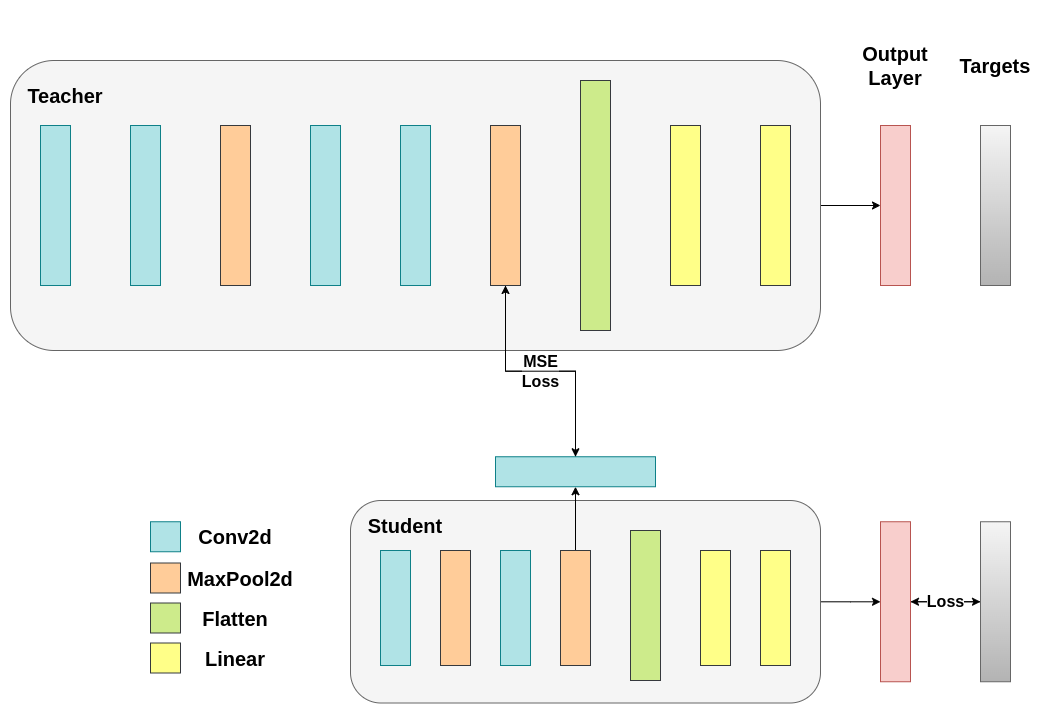
可训练层匹配中间张量的形状，并且均方误差 (MSE) 被正确定义：

class ModifiedDeepNNRegressor(nn.Module):
    def __init__(self, num_classes=10):
        super(ModifiedDeepNNRegressor, self).__init__()
        self.features = nn.Sequential(
            nn.Conv2d(3, 128, kernel_size=3, padding=1),
            nn.ReLU(),
            nn.Conv2d(128, 64, kernel_size=3, padding=1),
            nn.ReLU(),
            nn.MaxPool2d(kernel_size=2, stride=2),
            nn.Conv2d(64, 64, kernel_size=3, padding=1),
            nn.ReLU(),
            nn.Conv2d(64, 32, kernel_size=3, padding=1),
            nn.ReLU(),
            nn.MaxPool2d(kernel_size=2, stride=2),
        )
        self.classifier = nn.Sequential(
            nn.Linear(2048, 512),
            nn.ReLU(),
            nn.Dropout(0.1),
            nn.Linear(512, num_classes)
        )

    def forward(self, x):
        x = self.features(x)
        conv_feature_map = x
        x = torch.flatten(x, 1)
        x = self.classifier(x)
        return x, conv_feature_map

class ModifiedLightNNRegressor(nn.Module):
    def __init__(self, num_classes=10):
        super(ModifiedLightNNRegressor, self).__init__()
        self.features = nn.Sequential(
            nn.Conv2d(3, 16, kernel_size=3, padding=1),
            nn.ReLU(),
            nn.MaxPool2d(kernel_size=2, stride=2),
            nn.Conv2d(16, 16, kernel_size=3, padding=1),
            nn.ReLU(),
            nn.MaxPool2d(kernel_size=2, stride=2),
        )
        # Include an extra regressor (in our case linear)
        self.regressor = nn.Sequential(
            nn.Conv2d(16, 32, kernel_size=3, padding=1)
        )
        self.classifier = nn.Sequential(
            nn.Linear(1024, 256),
            nn.ReLU(),
            nn.Dropout(0.1),
            nn.Linear(256, num_classes)
        )

    def forward(self, x):
        x = self.features(x)
        regressor_output = self.regressor(x)
        x = torch.flatten(x, 1)
        x = self.classifier(x)
        return x, regressor_output

之后，我们必须再次更新我们的训练循环。这一次，我们提取学生网络的回归器输出和教师网络的特征图，计算这些张量的 MSE（它们的形状完全相同，因此定义正确），并在该损失的基础上反向传播梯度，此外还有分类任务的常规交叉熵损失。

def train_mse_loss(teacher, student, train_loader, epochs, learning_rate, feature_map_weight, ce_loss_weight, device):
    ce_loss = nn.CrossEntropyLoss()
    mse_loss = nn.MSELoss()
    optimizer = optim.Adam(student.parameters(), lr=learning_rate)

    teacher.to(device)
    student.to(device)
    teacher.eval()  # Teacher set to evaluation mode
    student.train() # Student to train mode

    for epoch in range(epochs):
        running_loss = 0.0
        for inputs, labels in train_loader:
            inputs, labels = inputs.to(device), labels.to(device)

            optimizer.zero_grad()

            # Again ignore teacher logits
            with torch.no_grad():
                _, teacher_feature_map = teacher(inputs)

            # Forward pass with the student model
            student_logits, regressor_feature_map = student(inputs)

            # Calculate the loss
            hidden_rep_loss = mse_loss(regressor_feature_map, teacher_feature_map)

            # Calculate the true label loss
            label_loss = ce_loss(student_logits, labels)

            # Weighted sum of the two losses
            loss = feature_map_weight * hidden_rep_loss + ce_loss_weight * label_loss

            loss.backward()
            optimizer.step()

            running_loss += loss.item()

        print(f"Epoch {epoch+1}/{epochs}, Loss: {running_loss / len(train_loader)}")

# Notice how our test function remains the same here with the one we used in our previous case. We only care about the actual outputs because we measure accuracy.

# Initialize a ModifiedLightNNRegressor
torch.manual_seed(42)
modified_nn_light_reg = ModifiedLightNNRegressor(num_classes=10).to(device)

# We do not have to train the modified deep network from scratch of course, we just load its weights from the trained instance
modified_nn_deep_reg = ModifiedDeepNNRegressor(num_classes=10).to(device)
modified_nn_deep_reg.load_state_dict(nn_deep.state_dict())

# Train and test once again
train_mse_loss(teacher=modified_nn_deep_reg, student=modified_nn_light_reg, train_loader=train_loader, epochs=10, learning_rate=0.001, feature_map_weight=0.25, ce_loss_weight=0.75, device=device)
test_accuracy_light_ce_and_mse_loss = test_multiple_outputs(modified_nn_light_reg, test_loader, device)

Epoch 1/10, Loss: 1.6814098352056634
Epoch 2/10, Loss: 1.3158039458267523
Epoch 3/10, Loss: 1.1743099965402841
Epoch 4/10, Loss: 1.0804673418059678
Epoch 5/10, Loss: 1.0056396507850998
Epoch 6/10, Loss: 0.9448006615004576
Epoch 7/10, Loss: 0.8926408891482731
Epoch 8/10, Loss: 0.842213883119471
Epoch 9/10, Loss: 0.8003371124682219
Epoch 10/10, Loss: 0.7620166893810263
Test Accuracy: 71.02%

预计最后一种方法会比 CosineLoss 效果更好，因为现在我们在教师网络和学生网络之间允许了一个可训练层，这给了学生网络一些学习的余地，而不是强制学生网络复制教师网络的表示。包含额外的网络是基于提示的蒸馏（hint-based distillation）背后的思想。

print(f"Teacher accuracy: {test_accuracy_deep:.2f}%")
print(f"Student accuracy without teacher: {test_accuracy_light_ce:.2f}%")
print(f"Student accuracy with CE + KD: {test_accuracy_light_ce_and_kd:.2f}%")
print(f"Student accuracy with CE + CosineLoss: {test_accuracy_light_ce_and_cosine_loss:.2f}%")
print(f"Student accuracy with CE + RegressorMSE: {test_accuracy_light_ce_and_mse_loss:.2f}%")

Teacher accuracy: 75.62%
Student accuracy without teacher: 70.43%
Student accuracy with CE + KD: 70.48%
Student accuracy with CE + CosineLoss: 70.76%
Student accuracy with CE + RegressorMSE: 71.02%

结论

上述方法均不会增加网络的参数数量或推理时间，因此性能提升的代价仅是在训练期间计算梯度所带来的微小开销。在机器学习应用中，我们主要关注推理时间，因为训练发生在模型部署之前。如果我们的轻量级模型对于部署仍然过重，我们可以应用不同的思路，例如训练后量化。附加损失可以应用于许多任务，而不仅仅是分类，并且你可以试验诸如系数（coefficients）、温度（temperature）或神经元数量（number of neurons）等量。欢迎调整上述教程中的任何数值，但请记住，如果你更改神经元/滤波器（filters）的数量，则很可能会发生形状不匹配（shape mismatch）。

更多信息请参阅：

• Hinton, G., Vinyals, O., Dean, J.: Distilling the knowledge in a neural network. In: Neural Information Processing System Deep Learning Workshop (2015)

• Romero, A., Ballas, N., Kahou, S.E., Chassang, A., Gatta, C., Bengio, Y.: Fitnets: Hints for thin deep nets. In: Proceedings of the International Conference on Learning Representations (2015)