计算机视觉迁移学习教程

创建日期: 2017 年 3 月 24 日 | 最后更新日期: 2025 年 1 月 27 日 | 最后验证日期: 2024 年 11 月 05 日

作者: Sasank Chilamkurthy

在本教程中，你将学习如何使用迁移学习训练一个用于图像分类的卷积神经网络。你可以在 cs231n 笔记中阅读更多关于迁移学习的内容。

引用这些笔记：

实际上，很少有人会从头开始训练一个完整的卷积网络（使用随机初始化），因为拥有足够大的数据集的情况相对罕见。相反，常见的做法是在一个非常大的数据集（例如 ImageNet，包含 120 万张图像和 1000 个类别）上预训练一个 ConvNet，然后将该 ConvNet 用作目标任务的初始化或固定特征提取器。

这两种主要的迁移学习场景如下：

• 微调 ConvNet：不是使用随机初始化，我们使用预训练的网络（例如在 imagenet 1000 数据集上训练的网络）初始化网络。其余的训练过程照常进行。

• 将 ConvNet 作为固定特征提取器：在这里，我们将冻结除了最终全连接层之外的所有网络权重。这个最后一个全连接层将被一个具有随机权重的新层取代，并且只训练这一层。

# License: BSD
# Author: Sasank Chilamkurthy

import torch
import torch.nn as nn
import torch.optim as optim
from torch.optim import lr_scheduler
import torch.backends.cudnn as cudnn
import numpy as np
import torchvision
from torchvision import datasets, models, transforms
import matplotlib.pyplot as plt
import time
import os
from PIL import Image
from tempfile import TemporaryDirectory

cudnn.benchmark = True
plt.ion()   # interactive mode

<contextlib.ExitStack object at 0x7f5645de7790>

加载数据

我们将使用 torchvision 和 torch.utils.data 包来加载数据。

我们今天将解决的问题是训练一个模型来分类蚂蚁和蜜蜂。我们有大约 120 张蚂蚁和蜜蜂的训练图像，每个类别各有约 120 张。每个类别有 75 张验证图像。通常，如果从头开始训练，这是一个非常小的数据集，难以进行泛化。由于我们使用迁移学习，我们应该能够相当好地泛化。

这个数据集是 imagenet 的一个非常小的子集。

注意

从此处下载数据并将其解压到当前目录。

# Data augmentation and normalization for training
# Just normalization for validation
data_transforms = {
    'train': transforms.Compose([
        transforms.RandomResizedCrop(224),
        transforms.RandomHorizontalFlip(),
        transforms.ToTensor(),
        transforms.Normalize([0.485, 0.456, 0.406], [0.229, 0.224, 0.225])
    ]),
    'val': transforms.Compose([
        transforms.Resize(256),
        transforms.CenterCrop(224),
        transforms.ToTensor(),
        transforms.Normalize([0.485, 0.456, 0.406], [0.229, 0.224, 0.225])
    ]),
}

data_dir = 'data/hymenoptera_data'
image_datasets = {x: datasets.ImageFolder(os.path.join(data_dir, x),
                                          data_transforms[x])
                  for x in ['train', 'val']}
dataloaders = {x: torch.utils.data.DataLoader(image_datasets[x], batch_size=4,
                                             shuffle=True, num_workers=4)
              for x in ['train', 'val']}
dataset_sizes = {x: len(image_datasets[x]) for x in ['train', 'val']}
class_names = image_datasets['train'].classes

# We want to be able to train our model on an `accelerator <https://pytorch.ac.cn/docs/stable/torch.html#accelerators>`__
# such as CUDA, MPS, MTIA, or XPU. If the current accelerator is available, we will use it. Otherwise, we use the CPU.

device = torch.accelerator.current_accelerator().type if torch.accelerator.is_available() else "cpu"
print(f"Using {device} device")

Using cuda device

可视化一些图像

让我们可视化一些训练图像，以便理解数据增强。

def imshow(inp, title=None):
    """Display image for Tensor."""
    inp = inp.numpy().transpose((1, 2, 0))
    mean = np.array([0.485, 0.456, 0.406])
    std = np.array([0.229, 0.224, 0.225])
    inp = std * inp + mean
    inp = np.clip(inp, 0, 1)
    plt.imshow(inp)
    if title is not None:
        plt.title(title)
    plt.pause(0.001)  # pause a bit so that plots are updated


# Get a batch of training data
inputs, classes = next(iter(dataloaders['train']))

# Make a grid from batch
out = torchvision.utils.make_grid(inputs)

imshow(out, title=[class_names[x] for x in classes])

训练模型

现在，让我们编写一个通用的函数来训练模型。这里我们将说明：

• 调度学习率

• 保存最佳模型

在下文中，参数 scheduler 是来自 torch.optim.lr_scheduler 的学习率调度器对象。

def train_model(model, criterion, optimizer, scheduler, num_epochs=25):
    since = time.time()

    # Create a temporary directory to save training checkpoints
    with TemporaryDirectory() as tempdir:
        best_model_params_path = os.path.join(tempdir, 'best_model_params.pt')

        torch.save(model.state_dict(), best_model_params_path)
        best_acc = 0.0

        for epoch in range(num_epochs):
            print(f'Epoch {epoch}/{num_epochs - 1}')
            print('-' * 10)

            # Each epoch has a training and validation phase
            for phase in ['train', 'val']:
                if phase == 'train':
                    model.train()  # Set model to training mode
                else:
                    model.eval()   # Set model to evaluate mode

                running_loss = 0.0
                running_corrects = 0

                # Iterate over data.
                for inputs, labels in dataloaders[phase]:
                    inputs = inputs.to(device)
                    labels = labels.to(device)

                    # zero the parameter gradients
                    optimizer.zero_grad()

                    # forward
                    # track history if only in train
                    with torch.set_grad_enabled(phase == 'train'):
                        outputs = model(inputs)
                        _, preds = torch.max(outputs, 1)
                        loss = criterion(outputs, labels)

                        # backward + optimize only if in training phase
                        if phase == 'train':
                            loss.backward()
                            optimizer.step()

                    # statistics
                    running_loss += loss.item() * inputs.size(0)
                    running_corrects += torch.sum(preds == labels.data)
                if phase == 'train':
                    scheduler.step()

                epoch_loss = running_loss / dataset_sizes[phase]
                epoch_acc = running_corrects.double() / dataset_sizes[phase]

                print(f'{phase} Loss: {epoch_loss:.4f} Acc: {epoch_acc:.4f}')

                # deep copy the model
                if phase == 'val' and epoch_acc > best_acc:
                    best_acc = epoch_acc
                    torch.save(model.state_dict(), best_model_params_path)

            print()

        time_elapsed = time.time() - since
        print(f'Training complete in {time_elapsed // 60:.0f}m {time_elapsed % 60:.0f}s')
        print(f'Best val Acc: {best_acc:4f}')

        # load best model weights
        model.load_state_dict(torch.load(best_model_params_path, weights_only=True))
    return model

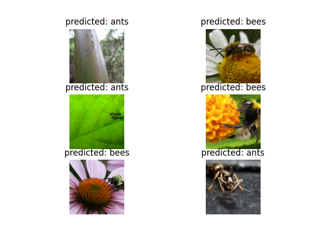
可视化模型预测

显示一些图像预测的通用函数

def visualize_model(model, num_images=6):
    was_training = model.training
    model.eval()
    images_so_far = 0
    fig = plt.figure()

    with torch.no_grad():
        for i, (inputs, labels) in enumerate(dataloaders['val']):
            inputs = inputs.to(device)
            labels = labels.to(device)

            outputs = model(inputs)
            _, preds = torch.max(outputs, 1)

            for j in range(inputs.size()[0]):
                images_so_far += 1
                ax = plt.subplot(num_images//2, 2, images_so_far)
                ax.axis('off')
                ax.set_title(f'predicted: {class_names[preds[j]]}')
                imshow(inputs.cpu().data[j])

                if images_so_far == num_images:
                    model.train(mode=was_training)
                    return
        model.train(mode=was_training)

微调 ConvNet

加载预训练模型并重置最终全连接层。

model_ft = models.resnet18(weights='IMAGENET1K_V1')
num_ftrs = model_ft.fc.in_features
# Here the size of each output sample is set to 2.
# Alternatively, it can be generalized to ``nn.Linear(num_ftrs, len(class_names))``.
model_ft.fc = nn.Linear(num_ftrs, 2)

model_ft = model_ft.to(device)

criterion = nn.CrossEntropyLoss()

# Observe that all parameters are being optimized
optimizer_ft = optim.SGD(model_ft.parameters(), lr=0.001, momentum=0.9)

# Decay LR by a factor of 0.1 every 7 epochs
exp_lr_scheduler = lr_scheduler.StepLR(optimizer_ft, step_size=7, gamma=0.1)

Downloading: "https://download.pytorch.org/models/resnet18-f37072fd.pth" to /var/lib/ci-user/.cache/torch/hub/checkpoints/resnet18-f37072fd.pth

  0%|          | 0.00/44.7M [00:00<?, ?B/s]
 65%|######5   | 29.2M/44.7M [00:00<00:00, 301MB/s]
100%|##########| 44.7M/44.7M [00:00<00:00, 335MB/s]

训练和评估

在 CPU 上大约需要 15-25 分钟。在 GPU 上则不到一分钟。

model_ft = train_model(model_ft, criterion, optimizer_ft, exp_lr_scheduler,
                       num_epochs=25)

Epoch 0/24
----------
train Loss: 0.4787 Acc: 0.7623
val Loss: 0.2826 Acc: 0.8824

Epoch 1/24
----------
train Loss: 0.5323 Acc: 0.7951
val Loss: 0.5748 Acc: 0.7712

Epoch 2/24
----------
train Loss: 0.4174 Acc: 0.8320
val Loss: 0.2629 Acc: 0.9150

Epoch 3/24
----------
train Loss: 0.5516 Acc: 0.7664
val Loss: 0.3715 Acc: 0.8693

Epoch 4/24
----------
train Loss: 0.3716 Acc: 0.8689
val Loss: 0.2691 Acc: 0.9020

Epoch 5/24
----------
train Loss: 0.4827 Acc: 0.7992
val Loss: 0.2696 Acc: 0.8824

Epoch 6/24
----------
train Loss: 0.3853 Acc: 0.8115
val Loss: 0.4517 Acc: 0.8366

Epoch 7/24
----------
train Loss: 0.3616 Acc: 0.8607
val Loss: 0.2149 Acc: 0.9216

Epoch 8/24
----------
train Loss: 0.2117 Acc: 0.9098
val Loss: 0.2153 Acc: 0.9216

Epoch 9/24
----------
train Loss: 0.2672 Acc: 0.8770
val Loss: 0.2565 Acc: 0.8954

Epoch 10/24
----------
train Loss: 0.3424 Acc: 0.8525
val Loss: 0.2022 Acc: 0.9281

Epoch 11/24
----------
train Loss: 0.3070 Acc: 0.8402
val Loss: 0.2594 Acc: 0.9085

Epoch 12/24
----------
train Loss: 0.2223 Acc: 0.8975
val Loss: 0.2480 Acc: 0.9020

Epoch 13/24
----------
train Loss: 0.3150 Acc: 0.8648
val Loss: 0.1974 Acc: 0.9216

Epoch 14/24
----------
train Loss: 0.2537 Acc: 0.9098
val Loss: 0.2640 Acc: 0.9150

Epoch 15/24
----------
train Loss: 0.2886 Acc: 0.8689
val Loss: 0.3004 Acc: 0.9150

Epoch 16/24
----------
train Loss: 0.2168 Acc: 0.8934
val Loss: 0.2329 Acc: 0.9085

Epoch 17/24
----------
train Loss: 0.2331 Acc: 0.9098
val Loss: 0.1952 Acc: 0.9216

Epoch 18/24
----------
train Loss: 0.2578 Acc: 0.9139
val Loss: 0.2462 Acc: 0.9150

Epoch 19/24
----------
train Loss: 0.2068 Acc: 0.9139
val Loss: 0.2290 Acc: 0.9085

Epoch 20/24
----------
train Loss: 0.2569 Acc: 0.8689
val Loss: 0.2089 Acc: 0.9085

Epoch 21/24
----------
train Loss: 0.2562 Acc: 0.8975
val Loss: 0.2546 Acc: 0.9150

Epoch 22/24
----------
train Loss: 0.3195 Acc: 0.8484
val Loss: 0.2214 Acc: 0.8954

Epoch 23/24
----------
train Loss: 0.2553 Acc: 0.8893
val Loss: 0.2295 Acc: 0.9150

Epoch 24/24
----------
train Loss: 0.2891 Acc: 0.8811
val Loss: 0.2033 Acc: 0.9216

Training complete in 0m 35s
Best val Acc: 0.928105

visualize_model(model_ft)

将 ConvNet 作为固定特征提取器

在这里，我们需要冻结除了最后一层之外的所有网络。我们需要设置 requires_grad = False 来冻结参数，以便在 backward() 中不计算梯度。

你可以在此处的文档中阅读更多相关内容。

model_conv = torchvision.models.resnet18(weights='IMAGENET1K_V1')
for param in model_conv.parameters():
    param.requires_grad = False

# Parameters of newly constructed modules have requires_grad=True by default
num_ftrs = model_conv.fc.in_features
model_conv.fc = nn.Linear(num_ftrs, 2)

model_conv = model_conv.to(device)

criterion = nn.CrossEntropyLoss()

# Observe that only parameters of final layer are being optimized as
# opposed to before.
optimizer_conv = optim.SGD(model_conv.fc.parameters(), lr=0.001, momentum=0.9)

# Decay LR by a factor of 0.1 every 7 epochs
exp_lr_scheduler = lr_scheduler.StepLR(optimizer_conv, step_size=7, gamma=0.1)

训练和评估

在 CPU 上，这大约是前一种情况所需时间的一半。这是预期的，因为大多数网络不需要计算梯度。然而，前向传播仍然需要计算。

model_conv = train_model(model_conv, criterion, optimizer_conv,
                         exp_lr_scheduler, num_epochs=25)

Epoch 0/24
----------
train Loss: 0.6996 Acc: 0.6516
val Loss: 0.2014 Acc: 0.9346

Epoch 1/24
----------
train Loss: 0.4233 Acc: 0.8033
val Loss: 0.2655 Acc: 0.8758

Epoch 2/24
----------
train Loss: 0.4603 Acc: 0.7869
val Loss: 0.1847 Acc: 0.9477

Epoch 3/24
----------
train Loss: 0.3096 Acc: 0.8566
val Loss: 0.1747 Acc: 0.9477

Epoch 4/24
----------
train Loss: 0.4427 Acc: 0.8156
val Loss: 0.1630 Acc: 0.9477

Epoch 5/24
----------
train Loss: 0.5505 Acc: 0.7828
val Loss: 0.1642 Acc: 0.9477

Epoch 6/24
----------
train Loss: 0.3004 Acc: 0.8607
val Loss: 0.1744 Acc: 0.9542

Epoch 7/24
----------
train Loss: 0.4083 Acc: 0.8361
val Loss: 0.1892 Acc: 0.9412

Epoch 8/24
----------
train Loss: 0.4483 Acc: 0.7910
val Loss: 0.1984 Acc: 0.9477

Epoch 9/24
----------
train Loss: 0.3335 Acc: 0.8279
val Loss: 0.1942 Acc: 0.9412

Epoch 10/24
----------
train Loss: 0.2413 Acc: 0.8934
val Loss: 0.2000 Acc: 0.9477

Epoch 11/24
----------
train Loss: 0.3107 Acc: 0.8689
val Loss: 0.1801 Acc: 0.9412

Epoch 12/24
----------
train Loss: 0.3032 Acc: 0.8689
val Loss: 0.1669 Acc: 0.9477

Epoch 13/24
----------
train Loss: 0.3586 Acc: 0.8525
val Loss: 0.1900 Acc: 0.9477

Epoch 14/24
----------
train Loss: 0.2771 Acc: 0.8893
val Loss: 0.2318 Acc: 0.9216

Epoch 15/24
----------
train Loss: 0.3064 Acc: 0.8852
val Loss: 0.1909 Acc: 0.9477

Epoch 16/24
----------
train Loss: 0.4243 Acc: 0.8238
val Loss: 0.2227 Acc: 0.9346

Epoch 17/24
----------
train Loss: 0.3297 Acc: 0.8238
val Loss: 0.1916 Acc: 0.9412

Epoch 18/24
----------
train Loss: 0.4235 Acc: 0.8238
val Loss: 0.1766 Acc: 0.9477

Epoch 19/24
----------
train Loss: 0.2500 Acc: 0.8934
val Loss: 0.2003 Acc: 0.9477

Epoch 20/24
----------
train Loss: 0.2412 Acc: 0.8934
val Loss: 0.1821 Acc: 0.9477

Epoch 21/24
----------
train Loss: 0.3762 Acc: 0.8115
val Loss: 0.1842 Acc: 0.9412

Epoch 22/24
----------
train Loss: 0.3485 Acc: 0.8566
val Loss: 0.2166 Acc: 0.9281

Epoch 23/24
----------
train Loss: 0.3625 Acc: 0.8361
val Loss: 0.1747 Acc: 0.9412

Epoch 24/24
----------
train Loss: 0.3839 Acc: 0.8320
val Loss: 0.1768 Acc: 0.9412

Training complete in 0m 28s
Best val Acc: 0.954248

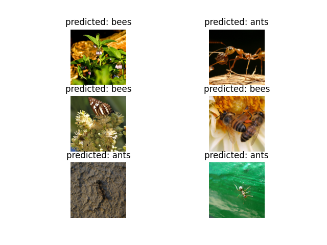
visualize_model(model_conv)

plt.ioff()
plt.show()

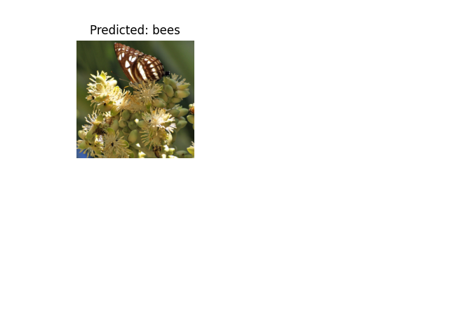
对自定义图像进行推理

使用训练好的模型对自定义图像进行预测，并可视化预测的类别标签以及图像。

def visualize_model_predictions(model,img_path):
    was_training = model.training
    model.eval()

    img = Image.open(img_path)
    img = data_transforms['val'](img)
    img = img.unsqueeze(0)
    img = img.to(device)

    with torch.no_grad():
        outputs = model(img)
        _, preds = torch.max(outputs, 1)

        ax = plt.subplot(2,2,1)
        ax.axis('off')
        ax.set_title(f'Predicted: {class_names[preds[0]]}')
        imshow(img.cpu().data[0])

        model.train(mode=was_training)

visualize_model_predictions(
    model_conv,
    img_path='data/hymenoptera_data/val/bees/72100438_73de9f17af.jpg'
)

plt.ioff()
plt.show()

进一步学习

如果你想了解更多关于迁移学习的应用，请查看我们的计算机视觉量化迁移学习教程。