


注意
点击这里下载完整的示例代码
空间变换网络教程
创建日期:2017 年 11 月 08 日 | 最后更新:2024 年 01 月 19 日 | 最后验证:2024 年 11 月 05 日

在本教程中,您将学习如何使用称为空间变换网络 (spatial transformer networks) 的视觉注意力机制来增强您的网络。您可以在 DeepMind 论文中阅读有关空间变换网络的更多信息
空间变换网络是可微分注意力对任何空间变换的推广。空间变换网络(简称 STN)允许神经网络学习如何对输入图像执行空间变换,以增强模型的几何不变性。例如,它可以裁剪感兴趣区域、缩放并校正图像的方向。这是一个有用的机制,因为 CNN 对旋转、缩放以及更一般的仿射变换并不具有不变性。
STN 最好的特点之一是能够非常轻松地将其插入任何现有的 CNN 中,只需进行少量修改。
# License: BSD
# Author: Ghassen Hamrouni

import torch
import torch.nn as nn
import torch.nn.functional as F
import torch.optim as optim
import torchvision
from torchvision import datasets, transforms
import matplotlib.pyplot as plt
import numpy as np

plt.ion()   # interactive mode
<contextlib.ExitStack object at 0x7ff915ba7280>
加载数据
在本文中,我们使用经典的 MNIST 数据集进行实验。使用一个用空间变换网络增强的标准卷积网络。
from six.moves import urllib
opener = urllib.request.build_opener()
opener.addheaders = [('User-agent', 'Mozilla/5.0')]
urllib.request.install_opener(opener)

device = torch.device("cuda" if torch.cuda.is_available() else "cpu")

# Training dataset
train_loader = torch.utils.data.DataLoader(
    datasets.MNIST(root='.', train=True, download=True,
                   transform=transforms.Compose([
                       transforms.ToTensor(),
                       transforms.Normalize((0.1307,), (0.3081,))
                   ])), batch_size=64, shuffle=True, num_workers=4)
# Test dataset
test_loader = torch.utils.data.DataLoader(
    datasets.MNIST(root='.', train=False, transform=transforms.Compose([
        transforms.ToTensor(),
        transforms.Normalize((0.1307,), (0.3081,))
    ])), batch_size=64, shuffle=True, num_workers=4)
  0%|          | 0.00/9.91M [00:00<?, ?B/s]
100%|##########| 9.91M/9.91M [00:00<00:00, 131MB/s]

  0%|          | 0.00/28.9k [00:00<?, ?B/s]
100%|##########| 28.9k/28.9k [00:00<00:00, 45.3MB/s]

  0%|          | 0.00/1.65M [00:00<?, ?B/s]
100%|##########| 1.65M/1.65M [00:00<00:00, 259MB/s]

  0%|          | 0.00/4.54k [00:00<?, ?B/s]
100%|##########| 4.54k/4.54k [00:00<00:00, 33.4MB/s]
描绘空间变换网络
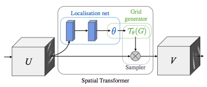
空间变换网络归结为三个主要组件
定位网络 (localization network) 是一个常规的 CNN,用于回归变换参数。这种变换并非从数据集中显式学习,而是网络自动学习能够提高全局准确性的空间变换。
网格生成器 (grid generator) 在输入图像中生成对应于输出图像中每个像素的坐标网格。
采样器 (sampler) 使用变换的参数并将其应用于输入图像。
注意
我们需要包含 affine_grid 和 grid_sample 模块的最新版 PyTorch。
class Net(nn.Module):
    def __init__(self):
        super(Net, self).__init__()
        self.conv1 = nn.Conv2d(1, 10, kernel_size=5)
        self.conv2 = nn.Conv2d(10, 20, kernel_size=5)
        self.conv2_drop = nn.Dropout2d()
        self.fc1 = nn.Linear(320, 50)
        self.fc2 = nn.Linear(50, 10)

        # Spatial transformer localization-network
        self.localization = nn.Sequential(
            nn.Conv2d(1, 8, kernel_size=7),
            nn.MaxPool2d(2, stride=2),
            nn.ReLU(True),
            nn.Conv2d(8, 10, kernel_size=5),
            nn.MaxPool2d(2, stride=2),
            nn.ReLU(True)
        )

        # Regressor for the 3 * 2 affine matrix
        self.fc_loc = nn.Sequential(
            nn.Linear(10 * 3 * 3, 32),
            nn.ReLU(True),
            nn.Linear(32, 3 * 2)
        )

        # Initialize the weights/bias with identity transformation
        self.fc_loc[2].weight.data.zero_()
        self.fc_loc[2].bias.data.copy_(torch.tensor([1, 0, 0, 0, 1, 0], dtype=torch.float))

    # Spatial transformer network forward function
    def stn(self, x):
        xs = self.localization(x)
        xs = xs.view(-1, 10 * 3 * 3)
        theta = self.fc_loc(xs)
        theta = theta.view(-1, 2, 3)

        grid = F.affine_grid(theta, x.size())
        x = F.grid_sample(x, grid)

        return x

    def forward(self, x):
        # transform the input
        x = self.stn(x)

        # Perform the usual forward pass
        x = F.relu(F.max_pool2d(self.conv1(x), 2))
        x = F.relu(F.max_pool2d(self.conv2_drop(self.conv2(x)), 2))
        x = x.view(-1, 320)
        x = F.relu(self.fc1(x))
        x = F.dropout(x, training=self.training)
        x = self.fc2(x)
        return F.log_softmax(x, dim=1)


model = Net().to(device)
训练模型
现在,让我们使用 SGD 算法来训练模型。网络正在以监督方式学习分类任务。同时,模型正在以端到端的方式自动学习 STN。
optimizer = optim.SGD(model.parameters(), lr=0.01)


def train(epoch):
    model.train()
    for batch_idx, (data, target) in enumerate(train_loader):
        data, target = data.to(device), target.to(device)

        optimizer.zero_grad()
        output = model(data)
        loss = F.nll_loss(output, target)
        loss.backward()
        optimizer.step()
        if batch_idx % 500 == 0:
            print('Train Epoch: {} [{}/{} ({:.0f}%)]\tLoss: {:.6f}'.format(
                epoch, batch_idx * len(data), len(train_loader.dataset),
                100. * batch_idx / len(train_loader), loss.item()))
#
# A simple test procedure to measure the STN performances on MNIST.
#


def test():
    with torch.no_grad():
        model.eval()
        test_loss = 0
        correct = 0
        for data, target in test_loader:
            data, target = data.to(device), target.to(device)
            output = model(data)

            # sum up batch loss
            test_loss += F.nll_loss(output, target, size_average=False).item()
            # get the index of the max log-probability
            pred = output.max(1, keepdim=True)[1]
            correct += pred.eq(target.view_as(pred)).sum().item()

        test_loss /= len(test_loader.dataset)
        print('\nTest set: Average loss: {:.4f}, Accuracy: {}/{} ({:.0f}%)\n'
              .format(test_loss, correct, len(test_loader.dataset),
                      100. * correct / len(test_loader.dataset)))
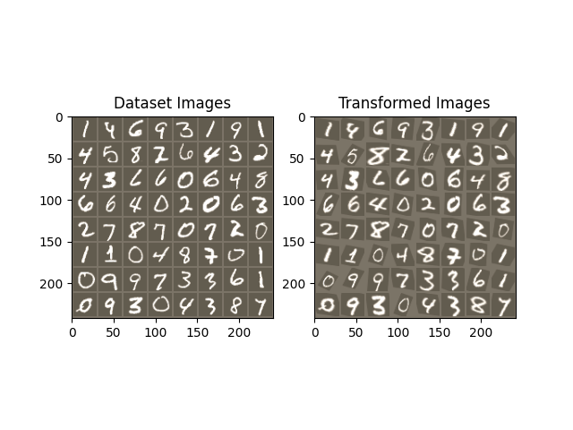
可视化 STN 结果
现在,我们将检查我们学习到的视觉注意力机制的结果。
我们定义了一个小的辅助函数,以便在训练期间可视化变换。
def convert_image_np(inp):
    """Convert a Tensor to numpy image."""
    inp = inp.numpy().transpose((1, 2, 0))
    mean = np.array([0.485, 0.456, 0.406])
    std = np.array([0.229, 0.224, 0.225])
    inp = std * inp + mean
    inp = np.clip(inp, 0, 1)
    return inp

# We want to visualize the output of the spatial transformers layer
# after the training, we visualize a batch of input images and
# the corresponding transformed batch using STN.


def visualize_stn():
    with torch.no_grad():
        # Get a batch of training data
        data = next(iter(test_loader))[0].to(device)

        input_tensor = data.cpu()
        transformed_input_tensor = model.stn(data).cpu()

        in_grid = convert_image_np(
            torchvision.utils.make_grid(input_tensor))

        out_grid = convert_image_np(
            torchvision.utils.make_grid(transformed_input_tensor))

        # Plot the results side-by-side
        f, axarr = plt.subplots(1, 2)
        axarr[0].imshow(in_grid)
        axarr[0].set_title('Dataset Images')

        axarr[1].imshow(out_grid)
        axarr[1].set_title('Transformed Images')

for epoch in range(1, 20 + 1):
    train(epoch)
    test()

# Visualize the STN transformation on some input batch
visualize_stn()

plt.ioff()
plt.show()
/var/lib/ci-user/.local/lib/python3.10/site-packages/torch/nn/functional.py:5082: UserWarning:

Default grid_sample and affine_grid behavior has changed to align_corners=False since 1.3.0. Please specify align_corners=True if the old behavior is desired. See the documentation of grid_sample for details.

/var/lib/ci-user/.local/lib/python3.10/site-packages/torch/nn/functional.py:5015: UserWarning:

Default grid_sample and affine_grid behavior has changed to align_corners=False since 1.3.0. Please specify align_corners=True if the old behavior is desired. See the documentation of grid_sample for details.

Train Epoch: 1 [0/60000 (0%)]   Loss: 2.315653
Train Epoch: 1 [32000/60000 (53%)]      Loss: 1.101937
/var/lib/ci-user/.local/lib/python3.10/site-packages/torch/nn/_reduction.py:51: UserWarning:

size_average and reduce args will be deprecated, please use reduction='sum' instead.


Test set: Average loss: 0.3017, Accuracy: 9121/10000 (91%)

Train Epoch: 2 [0/60000 (0%)]   Loss: 0.617127
Train Epoch: 2 [32000/60000 (53%)]      Loss: 0.336211

Test set: Average loss: 0.1752, Accuracy: 9484/10000 (95%)

Train Epoch: 3 [0/60000 (0%)]   Loss: 0.302927
Train Epoch: 3 [32000/60000 (53%)]      Loss: 0.209457

Test set: Average loss: 0.1162, Accuracy: 9657/10000 (97%)

Train Epoch: 4 [0/60000 (0%)]   Loss: 0.357578
Train Epoch: 4 [32000/60000 (53%)]      Loss: 0.133743

Test set: Average loss: 0.0980, Accuracy: 9700/10000 (97%)

Train Epoch: 5 [0/60000 (0%)]   Loss: 0.200890
Train Epoch: 5 [32000/60000 (53%)]      Loss: 0.181845

Test set: Average loss: 0.5375, Accuracy: 8342/10000 (83%)

Train Epoch: 6 [0/60000 (0%)]   Loss: 1.124530
Train Epoch: 6 [32000/60000 (53%)]      Loss: 0.153496

Test set: Average loss: 0.0761, Accuracy: 9776/10000 (98%)

Train Epoch: 7 [0/60000 (0%)]   Loss: 0.103622
Train Epoch: 7 [32000/60000 (53%)]      Loss: 0.201051

Test set: Average loss: 0.0846, Accuracy: 9753/10000 (98%)

Train Epoch: 8 [0/60000 (0%)]   Loss: 0.211345
Train Epoch: 8 [32000/60000 (53%)]      Loss: 0.051029

Test set: Average loss: 0.0811, Accuracy: 9757/10000 (98%)

Train Epoch: 9 [0/60000 (0%)]   Loss: 0.071642
Train Epoch: 9 [32000/60000 (53%)]      Loss: 0.133627

Test set: Average loss: 0.0690, Accuracy: 9780/10000 (98%)

Train Epoch: 10 [0/60000 (0%)]  Loss: 0.092827
Train Epoch: 10 [32000/60000 (53%)]     Loss: 0.260080

Test set: Average loss: 0.0623, Accuracy: 9813/10000 (98%)

Train Epoch: 11 [0/60000 (0%)]  Loss: 0.181832
Train Epoch: 11 [32000/60000 (53%)]     Loss: 0.095419

Test set: Average loss: 0.0569, Accuracy: 9826/10000 (98%)

Train Epoch: 12 [0/60000 (0%)]  Loss: 0.101949
Train Epoch: 12 [32000/60000 (53%)]     Loss: 0.123148

Test set: Average loss: 0.0531, Accuracy: 9838/10000 (98%)

Train Epoch: 13 [0/60000 (0%)]  Loss: 0.079982
Train Epoch: 13 [32000/60000 (53%)]     Loss: 0.097950

Test set: Average loss: 0.0617, Accuracy: 9815/10000 (98%)

Train Epoch: 14 [0/60000 (0%)]  Loss: 0.051012
Train Epoch: 14 [32000/60000 (53%)]     Loss: 0.142395

Test set: Average loss: 0.0536, Accuracy: 9841/10000 (98%)

Train Epoch: 15 [0/60000 (0%)]  Loss: 0.038217
Train Epoch: 15 [32000/60000 (53%)]     Loss: 0.055030

Test set: Average loss: 0.0503, Accuracy: 9843/10000 (98%)

Train Epoch: 16 [0/60000 (0%)]  Loss: 0.036684
Train Epoch: 16 [32000/60000 (53%)]     Loss: 0.136846

Test set: Average loss: 0.0462, Accuracy: 9863/10000 (99%)

Train Epoch: 17 [0/60000 (0%)]  Loss: 0.278311
Train Epoch: 17 [32000/60000 (53%)]     Loss: 0.318396

Test set: Average loss: 0.0475, Accuracy: 9856/10000 (99%)

Train Epoch: 18 [0/60000 (0%)]  Loss: 0.044018
Train Epoch: 18 [32000/60000 (53%)]     Loss: 0.067962

Test set: Average loss: 0.0471, Accuracy: 9864/10000 (99%)

Train Epoch: 19 [0/60000 (0%)]  Loss: 0.050557
Train Epoch: 19 [32000/60000 (53%)]     Loss: 0.111027

Test set: Average loss: 0.0569, Accuracy: 9831/10000 (98%)

Train Epoch: 20 [0/60000 (0%)]  Loss: 0.120847
Train Epoch: 20 [32000/60000 (53%)]     Loss: 0.037086

Test set: Average loss: 0.0620, Accuracy: 9807/10000 (98%)
脚本总运行时间: ( 1 分 34.935 秒)
