注意

点击此处下载完整示例代码

TorchVision 目标检测微调教程¶

创建日期：2023 年 12 月 14 日 | 最后更新：2024 年 6 月 11 日 | 最后验证：2024 年 11 月 5 日

在本教程中，我们将使用 Mask R-CNN 预训练模型在 Penn-Fudan 行人检测和分割数据集上进行微调。该数据集包含 170 张图像和 345 个行人实例，我们将使用它来演示如何利用 torchvision 中的新功能在自定义数据集上训练目标检测和实例分割模型。

注意

本教程仅适用于 torchvision 版本 >=0.16 或 nightly 版本。如果您使用的是 torchvision<=0.15 版本，请改为遵循此教程。

定义数据集¶

用于训练目标检测、实例分割和人体关键点检测的参考脚本可以轻松支持添加新的自定义数据集。数据集应继承标准 torch.utils.data.Dataset 类，并实现 __len__ 和 __getitem__ 方法。

我们唯一的要求是数据集的 __getitem__ 方法应返回一个元组

image：形状为 [3, H, W] 的 torchvision.tv_tensors.Image，一个纯张量，或大小为 (H, W) 的 PIL 图像
target：一个包含以下字段的字典
- boxes，形状为 [N, 4] 的 torchvision.tv_tensors.BoundingBoxes：N 个边界框的坐标，格式为 [x0, y0, x1, y1]，范围从 0 到 W，从 0 到 H
- labels，形状为 [N] 的整型 torch.Tensor：每个边界框的标签。0 始终表示背景类。
- image_id，整型：图像标识符。在数据集中的所有图像之间应是唯一的，用于评估期间
- area，形状为 [N] 的浮点型 torch.Tensor：边界框的面积。这在 COCO 指标评估期间用于区分小型、中型和大型框的指标得分。
- iscrowd，形状为 [N] 的 uint8 torch.Tensor：iscrowd=True 的实例在评估期间将被忽略。
- (可选) masks，形状为 [N, H, W] 的 torchvision.tv_tensors.Mask：每个对象的分割掩码

如果您的数据集符合上述要求，那么它将适用于参考脚本中的训练和评估代码。评估代码将使用 pycocotools 的脚本，可以使用 pip install pycocotools 安装。

注意

对于 Windows，请使用以下命令从 gautamchitnis 安装 pycocotools

pip install git+https://github.com/gautamchitnis/cocoapi.git@cocodataset-master#subdirectory=PythonAPI

关于 labels 的一个注意事项。模型将类别 0 视为背景。如果您的数据集不包含背景类别，则您的 labels 中不应包含 0。例如，假设您只有两个类别，猫和狗，您可以定义 1（不是 0）来表示猫，定义 2 来表示狗。因此，例如，如果某张图像同时包含这两个类别，您的 labels 张量应类似于 [1, 2]。

此外，如果您想在训练期间使用纵横比分组（以便每个批次仅包含具有相似纵横比的图像），那么还建议实现一个 get_height_and_width 方法，该方法返回图像的高度和宽度。如果未提供此方法，我们将通过 __getitem__ 查询数据集的所有元素，这将图像加载到内存中，比提供自定义方法要慢。

为 PennFudan 编写自定义数据集¶

让我们为 PennFudan 数据集编写一个数据集。首先，让我们下载数据集并解压 zip 文件

wget https://www.cis.upenn.edu/~jshi/ped_html/PennFudanPed.zip -P data
cd data && unzip PennFudanPed.zip

我们有以下文件夹结构

PennFudanPed/
  PedMasks/
    FudanPed00001_mask.png
    FudanPed00002_mask.png
    FudanPed00003_mask.png
    FudanPed00004_mask.png
    ...
  PNGImages/
    FudanPed00001.png
    FudanPed00002.png
    FudanPed00003.png
    FudanPed00004.png

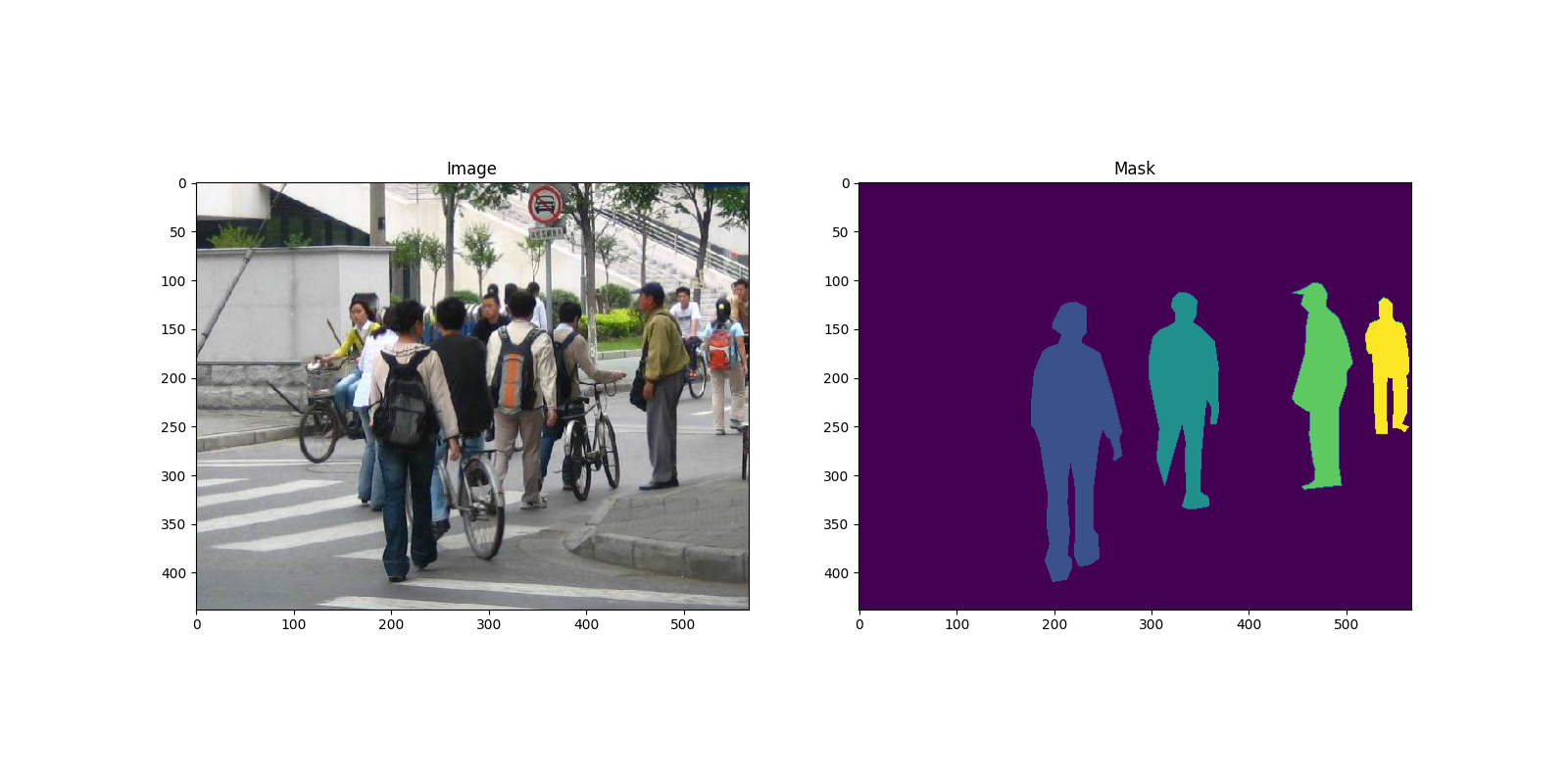
这是一对图像和分割掩码的示例

import matplotlib.pyplot as plt
from torchvision.io import read_image


image = read_image("data/PennFudanPed/PNGImages/FudanPed00046.png")
mask = read_image("data/PennFudanPed/PedMasks/FudanPed00046_mask.png")

plt.figure(figsize=(16, 8))
plt.subplot(121)
plt.title("Image")
plt.imshow(image.permute(1, 2, 0))
plt.subplot(122)
plt.title("Mask")
plt.imshow(mask.permute(1, 2, 0))

<matplotlib.image.AxesImage object at 0x7f28154b8fa0>

因此，每张图像都有对应的分割掩码，其中每种颜色对应一个不同的实例。让我们为该数据集编写一个 torch.utils.data.Dataset 类。在下面的代码中，我们将图像、边界框和掩码包装到 torchvision.tv_tensors.TVTensor 类中，以便能够为给定的目标检测和分割任务应用 torchvision 内置变换（新的 Transforms API）。具体来说，图像张量将被 torchvision.tv_tensors.Image 包装，边界框将被 torchvision.tv_tensors.BoundingBoxes 包装，掩码将被 torchvision.tv_tensors.Mask 包装。由于 torchvision.tv_tensors.TVTensor 是 torch.Tensor 的子类，被包装的对象也是张量，并继承了原生的 torch.Tensor API。有关 torchvision tv_tensors 的更多信息，请参阅此文档。

import os
import torch

from torchvision.io import read_image
from torchvision.ops.boxes import masks_to_boxes
from torchvision import tv_tensors
from torchvision.transforms.v2 import functional as F


class PennFudanDataset(torch.utils.data.Dataset):
    def __init__(self, root, transforms):
        self.root = root
        self.transforms = transforms
        # load all image files, sorting them to
        # ensure that they are aligned
        self.imgs = list(sorted(os.listdir(os.path.join(root, "PNGImages"))))
        self.masks = list(sorted(os.listdir(os.path.join(root, "PedMasks"))))

    def __getitem__(self, idx):
        # load images and masks
        img_path = os.path.join(self.root, "PNGImages", self.imgs[idx])
        mask_path = os.path.join(self.root, "PedMasks", self.masks[idx])
        img = read_image(img_path)
        mask = read_image(mask_path)
        # instances are encoded as different colors
        obj_ids = torch.unique(mask)
        # first id is the background, so remove it
        obj_ids = obj_ids[1:]
        num_objs = len(obj_ids)

        # split the color-encoded mask into a set
        # of binary masks
        masks = (mask == obj_ids[:, None, None]).to(dtype=torch.uint8)

        # get bounding box coordinates for each mask
        boxes = masks_to_boxes(masks)

        # there is only one class
        labels = torch.ones((num_objs,), dtype=torch.int64)

        image_id = idx
        area = (boxes[:, 3] - boxes[:, 1]) * (boxes[:, 2] - boxes[:, 0])
        # suppose all instances are not crowd
        iscrowd = torch.zeros((num_objs,), dtype=torch.int64)

        # Wrap sample and targets into torchvision tv_tensors:
        img = tv_tensors.Image(img)

        target = {}
        target["boxes"] = tv_tensors.BoundingBoxes(boxes, format="XYXY", canvas_size=F.get_size(img))
        target["masks"] = tv_tensors.Mask(masks)
        target["labels"] = labels
        target["image_id"] = image_id
        target["area"] = area
        target["iscrowd"] = iscrowd

        if self.transforms is not None:
            img, target = self.transforms(img, target)

        return img, target

    def __len__(self):
        return len(self.imgs)

数据集部分就到此为止。现在让我们定义一个可以在此数据集上执行预测的模型。

定义您的模型¶

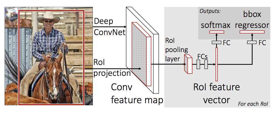
在本教程中，我们将使用基于 Faster R-CNN 的 Mask R-CNN。Faster R-CNN 是一种预测图像中潜在对象的边界框和类别得分的模型。

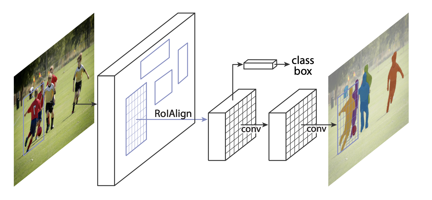
../_static/img/tv_tutorial/tv_image03.png

Mask R-CNN 在 Faster R-CNN 中添加了一个额外的分支，该分支也预测每个实例的分割掩码。

../_static/img/tv_tutorial/tv_image04.png

有两种常见的情况，用户可能希望修改 TorchVision 模型动物园中可用的模型之一。第一种情况是，我们希望从预训练模型开始，只对最后一层进行微调。另一种情况是，我们希望用不同的主干网络替换模型的主干（例如，为了更快的预测）。

让我们看看在以下部分中如何实现其中一种情况。

1 - 从预训练模型进行微调¶

假设您想从一个在 COCO 上预训练的模型开始，并想为您的特定类别对其进行微调。这是一种可能的方法

import torchvision
from torchvision.models.detection.faster_rcnn import FastRCNNPredictor

# load a model pre-trained on COCO
model = torchvision.models.detection.fasterrcnn_resnet50_fpn(weights="DEFAULT")

# replace the classifier with a new one, that has
# num_classes which is user-defined
num_classes = 2  # 1 class (person) + background
# get number of input features for the classifier
in_features = model.roi_heads.box_predictor.cls_score.in_features
# replace the pre-trained head with a new one
model.roi_heads.box_predictor = FastRCNNPredictor(in_features, num_classes)

Downloading: "https://download.pytorch.org/models/fasterrcnn_resnet50_fpn_coco-258fb6c6.pth" to /var/lib/ci-user/.cache/torch/hub/checkpoints/fasterrcnn_resnet50_fpn_coco-258fb6c6.pth

  0%|          | 0.00/160M [00:00<?, ?B/s]
 27%|##6       | 42.9M/160M [00:00<00:00, 449MB/s]
 54%|#####4    | 87.0M/160M [00:00<00:00, 457MB/s]
 82%|########2 | 131M/160M [00:00<00:00, 459MB/s]
100%|##########| 160M/160M [00:00<00:00, 458MB/s]

2 - 修改模型以添加不同的主干网络¶

import torchvision
from torchvision.models.detection import FasterRCNN
from torchvision.models.detection.rpn import AnchorGenerator

# load a pre-trained model for classification and return
# only the features
backbone = torchvision.models.mobilenet_v2(weights="DEFAULT").features
# ``FasterRCNN`` needs to know the number of
# output channels in a backbone. For mobilenet_v2, it's 1280
# so we need to add it here
backbone.out_channels = 1280

# let's make the RPN generate 5 x 3 anchors per spatial
# location, with 5 different sizes and 3 different aspect
# ratios. We have a Tuple[Tuple[int]] because each feature
# map could potentially have different sizes and
# aspect ratios
anchor_generator = AnchorGenerator(
    sizes=((32, 64, 128, 256, 512),),
    aspect_ratios=((0.5, 1.0, 2.0),)
)

# let's define what are the feature maps that we will
# use to perform the region of interest cropping, as well as
# the size of the crop after rescaling.
# if your backbone returns a Tensor, featmap_names is expected to
# be [0]. More generally, the backbone should return an
# ``OrderedDict[Tensor]``, and in ``featmap_names`` you can choose which
# feature maps to use.
roi_pooler = torchvision.ops.MultiScaleRoIAlign(
    featmap_names=['0'],
    output_size=7,
    sampling_ratio=2
)

# put the pieces together inside a Faster-RCNN model
model = FasterRCNN(
    backbone,
    num_classes=2,
    rpn_anchor_generator=anchor_generator,
    box_roi_pool=roi_pooler
)

Downloading: "https://download.pytorch.org/models/mobilenet_v2-7ebf99e0.pth" to /var/lib/ci-user/.cache/torch/hub/checkpoints/mobilenet_v2-7ebf99e0.pth

  0%|          | 0.00/13.6M [00:00<?, ?B/s]
100%|##########| 13.6M/13.6M [00:00<00:00, 401MB/s]

用于 PennFudan 数据集的目标检测和实例分割模型¶

在我们的例子中，由于我们的数据集非常小，我们希望从预训练模型进行微调，因此我们将遵循方法 1。

在这里，我们还希望计算实例分割掩码，因此我们将使用 Mask R-CNN

import torchvision
from torchvision.models.detection.faster_rcnn import FastRCNNPredictor
from torchvision.models.detection.mask_rcnn import MaskRCNNPredictor


def get_model_instance_segmentation(num_classes):
    # load an instance segmentation model pre-trained on COCO
    model = torchvision.models.detection.maskrcnn_resnet50_fpn(weights="DEFAULT")

    # get number of input features for the classifier
    in_features = model.roi_heads.box_predictor.cls_score.in_features
    # replace the pre-trained head with a new one
    model.roi_heads.box_predictor = FastRCNNPredictor(in_features, num_classes)

    # now get the number of input features for the mask classifier
    in_features_mask = model.roi_heads.mask_predictor.conv5_mask.in_channels
    hidden_layer = 256
    # and replace the mask predictor with a new one
    model.roi_heads.mask_predictor = MaskRCNNPredictor(
        in_features_mask,
        hidden_layer,
        num_classes
    )

    return model

就这样，这将使 model 准备好在您的自定义数据集上进行训练和评估。

整合所有内容¶

在 references/detection/ 中，我们有许多辅助函数来简化检测模型的训练和评估。在此，我们将使用 references/detection/engine.py 和 references/detection/utils.py。只需将 references/detection 下的所有内容下载到您的文件夹中即可在此处使用它们。在 Linux 上，如果您安装了 wget，可以使用以下命令下载它们

os.system("wget https://raw.githubusercontent.com/pytorch/vision/main/references/detection/engine.py")
os.system("wget https://raw.githubusercontent.com/pytorch/vision/main/references/detection/utils.py")
os.system("wget https://raw.githubusercontent.com/pytorch/vision/main/references/detection/coco_utils.py")
os.system("wget https://raw.githubusercontent.com/pytorch/vision/main/references/detection/coco_eval.py")
os.system("wget https://raw.githubusercontent.com/pytorch/vision/main/references/detection/transforms.py")

自 v0.15.0 起，torchvision 提供了新的 Transforms API，以便轻松编写用于目标检测和分割任务的数据增强流程。

让我们编写一些用于数据增强/变换的辅助函数

from torchvision.transforms import v2 as T


def get_transform(train):
    transforms = []
    if train:
        transforms.append(T.RandomHorizontalFlip(0.5))
    transforms.append(T.ToDtype(torch.float, scale=True))
    transforms.append(T.ToPureTensor())
    return T.Compose(transforms)

测试 `forward()` 方法 (可选)¶

在迭代数据集之前，最好先了解模型在训练和推理阶段对样本数据的期望。

import utils

model = torchvision.models.detection.fasterrcnn_resnet50_fpn(weights="DEFAULT")
dataset = PennFudanDataset('data/PennFudanPed', get_transform(train=True))
data_loader = torch.utils.data.DataLoader(
    dataset,
    batch_size=2,
    shuffle=True,
    collate_fn=utils.collate_fn
)

# For Training
images, targets = next(iter(data_loader))
images = list(image for image in images)
targets = [{k: v for k, v in t.items()} for t in targets]
output = model(images, targets)  # Returns losses and detections
print(output)

# For inference
model.eval()
x = [torch.rand(3, 300, 400), torch.rand(3, 500, 400)]
predictions = model(x)  # Returns predictions
print(predictions[0])

{'loss_classifier': tensor(0.0798, grad_fn=<NllLossBackward0>), 'loss_box_reg': tensor(0.0284, grad_fn=<DivBackward0>), 'loss_objectness': tensor(0.0186, grad_fn=<BinaryCrossEntropyWithLogitsBackward0>), 'loss_rpn_box_reg': tensor(0.0034, grad_fn=<DivBackward0>)}
{'boxes': tensor([], size=(0, 4), grad_fn=<StackBackward0>), 'labels': tensor([], dtype=torch.int64), 'scores': tensor([], grad_fn=<IndexBackward0>)}

现在让我们编写执行训练和验证的主函数

from engine import train_one_epoch, evaluate

# train on the GPU or on the CPU, if a GPU is not available
device = torch.device('cuda') if torch.cuda.is_available() else torch.device('cpu')

# our dataset has two classes only - background and person
num_classes = 2
# use our dataset and defined transformations
dataset = PennFudanDataset('data/PennFudanPed', get_transform(train=True))
dataset_test = PennFudanDataset('data/PennFudanPed', get_transform(train=False))

# split the dataset in train and test set
indices = torch.randperm(len(dataset)).tolist()
dataset = torch.utils.data.Subset(dataset, indices[:-50])
dataset_test = torch.utils.data.Subset(dataset_test, indices[-50:])

# define training and validation data loaders
data_loader = torch.utils.data.DataLoader(
    dataset,
    batch_size=2,
    shuffle=True,
    collate_fn=utils.collate_fn
)

data_loader_test = torch.utils.data.DataLoader(
    dataset_test,
    batch_size=1,
    shuffle=False,
    collate_fn=utils.collate_fn
)

# get the model using our helper function
model = get_model_instance_segmentation(num_classes)

# move model to the right device
model.to(device)

# construct an optimizer
params = [p for p in model.parameters() if p.requires_grad]
optimizer = torch.optim.SGD(
    params,
    lr=0.005,
    momentum=0.9,
    weight_decay=0.0005
)

# and a learning rate scheduler
lr_scheduler = torch.optim.lr_scheduler.StepLR(
    optimizer,
    step_size=3,
    gamma=0.1
)

# let's train it just for 2 epochs
num_epochs = 2

for epoch in range(num_epochs):
    # train for one epoch, printing every 10 iterations
    train_one_epoch(model, optimizer, data_loader, device, epoch, print_freq=10)
    # update the learning rate
    lr_scheduler.step()
    # evaluate on the test dataset
    evaluate(model, data_loader_test, device=device)

print("That's it!")

Downloading: "https://download.pytorch.org/models/maskrcnn_resnet50_fpn_coco-bf2d0c1e.pth" to /var/lib/ci-user/.cache/torch/hub/checkpoints/maskrcnn_resnet50_fpn_coco-bf2d0c1e.pth

  0%|          | 0.00/170M [00:00<?, ?B/s]
 16%|#5        | 26.9M/170M [00:00<00:00, 282MB/s]
 33%|###3      | 56.6M/170M [00:00<00:00, 299MB/s]
 53%|#####2    | 89.8M/170M [00:00<00:00, 321MB/s]
 74%|#######3  | 126M/170M [00:00<00:00, 342MB/s]
 93%|#########3| 158M/170M [00:00<00:00, 299MB/s]
100%|##########| 170M/170M [00:00<00:00, 312MB/s]
/var/lib/workspace/intermediate_source/engine.py:30: FutureWarning:

`torch.cuda.amp.autocast(args...)` is deprecated. Please use `torch.amp.autocast('cuda', args...)` instead.

Epoch: [0]  [ 0/60]  eta: 0:00:25  lr: 0.000090  loss: 4.9115 (4.9115)  loss_classifier: 0.4416 (0.4416)  loss_box_reg: 0.1060 (0.1060)  loss_mask: 4.3587 (4.3587)  loss_objectness: 0.0028 (0.0028)  loss_rpn_box_reg: 0.0023 (0.0023)  time: 0.4216  data: 0.0132  max mem: 2448
Epoch: [0]  [10/60]  eta: 0:00:11  lr: 0.000936  loss: 1.7695 (2.7698)  loss_classifier: 0.4166 (0.3556)  loss_box_reg: 0.3051 (0.2540)  loss_mask: 0.9490 (2.1319)  loss_objectness: 0.0219 (0.0214)  loss_rpn_box_reg: 0.0056 (0.0069)  time: 0.2317  data: 0.0148  max mem: 2602
Epoch: [0]  [20/60]  eta: 0:00:08  lr: 0.001783  loss: 0.8103 (1.7889)  loss_classifier: 0.2160 (0.2681)  loss_box_reg: 0.2063 (0.2329)  loss_mask: 0.3992 (1.2596)  loss_objectness: 0.0134 (0.0202)  loss_rpn_box_reg: 0.0076 (0.0080)  time: 0.2095  data: 0.0150  max mem: 2627
Epoch: [0]  [30/60]  eta: 0:00:06  lr: 0.002629  loss: 0.6839 (1.4258)  loss_classifier: 0.1412 (0.2258)  loss_box_reg: 0.2292 (0.2426)  loss_mask: 0.2600 (0.9285)  loss_objectness: 0.0134 (0.0191)  loss_rpn_box_reg: 0.0101 (0.0098)  time: 0.2124  data: 0.0161  max mem: 2789
Epoch: [0]  [40/60]  eta: 0:00:04  lr: 0.003476  loss: 0.5391 (1.2069)  loss_classifier: 0.0929 (0.1910)  loss_box_reg: 0.2444 (0.2353)  loss_mask: 0.2286 (0.7549)  loss_objectness: 0.0115 (0.0158)  loss_rpn_box_reg: 0.0118 (0.0098)  time: 0.2122  data: 0.0165  max mem: 2789
Epoch: [0]  [50/60]  eta: 0:00:02  lr: 0.004323  loss: 0.3647 (1.0415)  loss_classifier: 0.0587 (0.1629)  loss_box_reg: 0.1545 (0.2171)  loss_mask: 0.1620 (0.6391)  loss_objectness: 0.0027 (0.0132)  loss_rpn_box_reg: 0.0071 (0.0093)  time: 0.2073  data: 0.0159  max mem: 2789
Epoch: [0]  [59/60]  eta: 0:00:00  lr: 0.005000  loss: 0.3598 (0.9431)  loss_classifier: 0.0396 (0.1451)  loss_box_reg: 0.1279 (0.2052)  loss_mask: 0.1620 (0.5724)  loss_objectness: 0.0014 (0.0116)  loss_rpn_box_reg: 0.0064 (0.0089)  time: 0.2027  data: 0.0150  max mem: 2789
Epoch: [0] Total time: 0:00:12 (0.2121 s / it)
creating index...
index created!
Test:  [ 0/50]  eta: 0:00:04  model_time: 0.0795 (0.0795)  evaluator_time: 0.0072 (0.0072)  time: 0.0993  data: 0.0121  max mem: 2789
Test:  [49/50]  eta: 0:00:00  model_time: 0.0419 (0.0578)  evaluator_time: 0.0048 (0.0066)  time: 0.0641  data: 0.0096  max mem: 2789
Test: Total time: 0:00:03 (0.0756 s / it)
Averaged stats: model_time: 0.0419 (0.0578)  evaluator_time: 0.0048 (0.0066)
Accumulating evaluation results...
DONE (t=0.01s).
Accumulating evaluation results...
DONE (t=0.01s).
IoU metric: bbox
 Average Precision  (AP) @[ IoU=0.50:0.95 | area=   all | maxDets=100 ] = 0.628
 Average Precision  (AP) @[ IoU=0.50      | area=   all | maxDets=100 ] = 0.983
 Average Precision  (AP) @[ IoU=0.75      | area=   all | maxDets=100 ] = 0.850
 Average Precision  (AP) @[ IoU=0.50:0.95 | area= small | maxDets=100 ] = 0.288
 Average Precision  (AP) @[ IoU=0.50:0.95 | area=medium | maxDets=100 ] = 0.600
 Average Precision  (AP) @[ IoU=0.50:0.95 | area= large | maxDets=100 ] = 0.640
 Average Recall     (AR) @[ IoU=0.50:0.95 | area=   all | maxDets=  1 ] = 0.278
 Average Recall     (AR) @[ IoU=0.50:0.95 | area=   all | maxDets= 10 ] = 0.682
 Average Recall     (AR) @[ IoU=0.50:0.95 | area=   all | maxDets=100 ] = 0.682
 Average Recall     (AR) @[ IoU=0.50:0.95 | area= small | maxDets=100 ] = 0.367
 Average Recall     (AR) @[ IoU=0.50:0.95 | area=medium | maxDets=100 ] = 0.675
 Average Recall     (AR) @[ IoU=0.50:0.95 | area= large | maxDets=100 ] = 0.691
IoU metric: segm
 Average Precision  (AP) @[ IoU=0.50:0.95 | area=   all | maxDets=100 ] = 0.663
 Average Precision  (AP) @[ IoU=0.50      | area=   all | maxDets=100 ] = 0.978
 Average Precision  (AP) @[ IoU=0.75      | area=   all | maxDets=100 ] = 0.780
 Average Precision  (AP) @[ IoU=0.50:0.95 | area= small | maxDets=100 ] = 0.424
 Average Precision  (AP) @[ IoU=0.50:0.95 | area=medium | maxDets=100 ] = 0.494
 Average Precision  (AP) @[ IoU=0.50:0.95 | area= large | maxDets=100 ] = 0.680
 Average Recall     (AR) @[ IoU=0.50:0.95 | area=   all | maxDets=  1 ] = 0.291
 Average Recall     (AR) @[ IoU=0.50:0.95 | area=   all | maxDets= 10 ] = 0.719
 Average Recall     (AR) @[ IoU=0.50:0.95 | area=   all | maxDets=100 ] = 0.722
 Average Recall     (AR) @[ IoU=0.50:0.95 | area= small | maxDets=100 ] = 0.600
 Average Recall     (AR) @[ IoU=0.50:0.95 | area=medium | maxDets=100 ] = 0.658
 Average Recall     (AR) @[ IoU=0.50:0.95 | area= large | maxDets=100 ] = 0.732
Epoch: [1]  [ 0/60]  eta: 0:00:10  lr: 0.005000  loss: 0.2563 (0.2563)  loss_classifier: 0.0182 (0.0182)  loss_box_reg: 0.0584 (0.0584)  loss_mask: 0.1751 (0.1751)  loss_objectness: 0.0014 (0.0014)  loss_rpn_box_reg: 0.0032 (0.0032)  time: 0.1773  data: 0.0139  max mem: 2789
Epoch: [1]  [10/60]  eta: 0:00:10  lr: 0.005000  loss: 0.3312 (0.3719)  loss_classifier: 0.0454 (0.0522)  loss_box_reg: 0.1256 (0.1413)  loss_mask: 0.1609 (0.1682)  loss_objectness: 0.0007 (0.0020)  loss_rpn_box_reg: 0.0078 (0.0082)  time: 0.2093  data: 0.0161  max mem: 2789
Epoch: [1]  [20/60]  eta: 0:00:08  lr: 0.005000  loss: 0.3338 (0.3483)  loss_classifier: 0.0409 (0.0452)  loss_box_reg: 0.1195 (0.1171)  loss_mask: 0.1698 (0.1772)  loss_objectness: 0.0008 (0.0017)  loss_rpn_box_reg: 0.0067 (0.0071)  time: 0.2059  data: 0.0151  max mem: 2789
Epoch: [1]  [30/60]  eta: 0:00:06  lr: 0.005000  loss: 0.3047 (0.3296)  loss_classifier: 0.0336 (0.0449)  loss_box_reg: 0.0884 (0.1111)  loss_mask: 0.1486 (0.1651)  loss_objectness: 0.0011 (0.0017)  loss_rpn_box_reg: 0.0045 (0.0069)  time: 0.2041  data: 0.0151  max mem: 2789
Epoch: [1]  [40/60]  eta: 0:00:04  lr: 0.005000  loss: 0.3015 (0.3258)  loss_classifier: 0.0439 (0.0444)  loss_box_reg: 0.0884 (0.1057)  loss_mask: 0.1480 (0.1663)  loss_objectness: 0.0016 (0.0022)  loss_rpn_box_reg: 0.0052 (0.0072)  time: 0.2047  data: 0.0157  max mem: 2789
Epoch: [1]  [50/60]  eta: 0:00:02  lr: 0.005000  loss: 0.2767 (0.3147)  loss_classifier: 0.0346 (0.0426)  loss_box_reg: 0.0582 (0.0995)  loss_mask: 0.1551 (0.1639)  loss_objectness: 0.0014 (0.0021)  loss_rpn_box_reg: 0.0042 (0.0066)  time: 0.2043  data: 0.0148  max mem: 2789
Epoch: [1]  [59/60]  eta: 0:00:00  lr: 0.005000  loss: 0.2267 (0.3004)  loss_classifier: 0.0331 (0.0413)  loss_box_reg: 0.0511 (0.0931)  loss_mask: 0.1289 (0.1576)  loss_objectness: 0.0006 (0.0021)  loss_rpn_box_reg: 0.0034 (0.0064)  time: 0.2067  data: 0.0154  max mem: 2789
Epoch: [1] Total time: 0:00:12 (0.2053 s / it)
creating index...
index created!
Test:  [ 0/50]  eta: 0:00:02  model_time: 0.0407 (0.0407)  evaluator_time: 0.0038 (0.0038)  time: 0.0570  data: 0.0120  max mem: 2789
Test:  [49/50]  eta: 0:00:00  model_time: 0.0397 (0.0410)  evaluator_time: 0.0033 (0.0042)  time: 0.0549  data: 0.0096  max mem: 2789
Test: Total time: 0:00:02 (0.0562 s / it)
Averaged stats: model_time: 0.0397 (0.0410)  evaluator_time: 0.0033 (0.0042)
Accumulating evaluation results...
DONE (t=0.01s).
Accumulating evaluation results...
DONE (t=0.01s).
IoU metric: bbox
 Average Precision  (AP) @[ IoU=0.50:0.95 | area=   all | maxDets=100 ] = 0.742
 Average Precision  (AP) @[ IoU=0.50      | area=   all | maxDets=100 ] = 0.986
 Average Precision  (AP) @[ IoU=0.75      | area=   all | maxDets=100 ] = 0.919
 Average Precision  (AP) @[ IoU=0.50:0.95 | area= small | maxDets=100 ] = 0.433
 Average Precision  (AP) @[ IoU=0.50:0.95 | area=medium | maxDets=100 ] = 0.701
 Average Precision  (AP) @[ IoU=0.50:0.95 | area= large | maxDets=100 ] = 0.756
 Average Recall     (AR) @[ IoU=0.50:0.95 | area=   all | maxDets=  1 ] = 0.317
 Average Recall     (AR) @[ IoU=0.50:0.95 | area=   all | maxDets= 10 ] = 0.790
 Average Recall     (AR) @[ IoU=0.50:0.95 | area=   all | maxDets=100 ] = 0.790
 Average Recall     (AR) @[ IoU=0.50:0.95 | area= small | maxDets=100 ] = 0.433
 Average Recall     (AR) @[ IoU=0.50:0.95 | area=medium | maxDets=100 ] = 0.758
 Average Recall     (AR) @[ IoU=0.50:0.95 | area= large | maxDets=100 ] = 0.803
IoU metric: segm
 Average Precision  (AP) @[ IoU=0.50:0.95 | area=   all | maxDets=100 ] = 0.719
 Average Precision  (AP) @[ IoU=0.50      | area=   all | maxDets=100 ] = 0.983
 Average Precision  (AP) @[ IoU=0.75      | area=   all | maxDets=100 ] = 0.863
 Average Precision  (AP) @[ IoU=0.50:0.95 | area= small | maxDets=100 ] = 0.394
 Average Precision  (AP) @[ IoU=0.50:0.95 | area=medium | maxDets=100 ] = 0.554
 Average Precision  (AP) @[ IoU=0.50:0.95 | area= large | maxDets=100 ] = 0.737
 Average Recall     (AR) @[ IoU=0.50:0.95 | area=   all | maxDets=  1 ] = 0.310
 Average Recall     (AR) @[ IoU=0.50:0.95 | area=   all | maxDets= 10 ] = 0.764
 Average Recall     (AR) @[ IoU=0.50:0.95 | area=   all | maxDets=100 ] = 0.764
 Average Recall     (AR) @[ IoU=0.50:0.95 | area= small | maxDets=100 ] = 0.533
 Average Recall     (AR) @[ IoU=0.50:0.95 | area=medium | maxDets=100 ] = 0.683
 Average Recall     (AR) @[ IoU=0.50:0.95 | area= large | maxDets=100 ] = 0.779
That's it!

因此，经过一个 epoch 的训练后，我们获得了 COCO 风格的 mAP > 50，以及掩码 mAP 为 65。

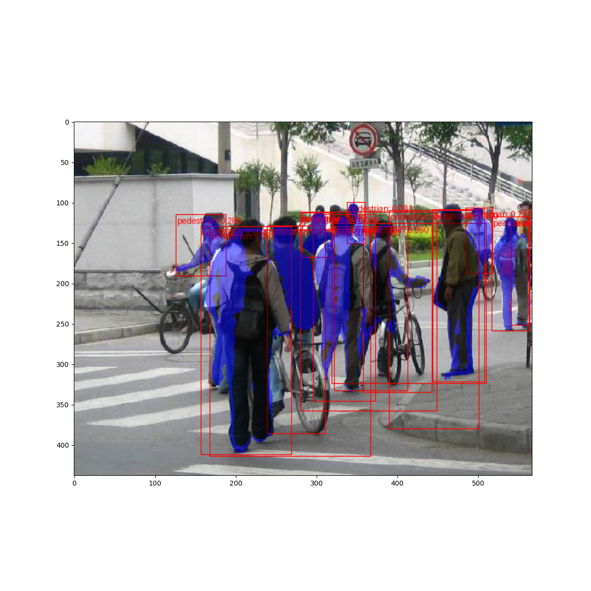
但是预测结果是什么样的呢？让我们从数据集中取一张图像进行验证

import matplotlib.pyplot as plt

from torchvision.utils import draw_bounding_boxes, draw_segmentation_masks


image = read_image("data/PennFudanPed/PNGImages/FudanPed00046.png")
eval_transform = get_transform(train=False)

model.eval()
with torch.no_grad():
    x = eval_transform(image)
    # convert RGBA -> RGB and move to device
    x = x[:3, ...].to(device)
    predictions = model([x, ])
    pred = predictions[0]


image = (255.0 * (image - image.min()) / (image.max() - image.min())).to(torch.uint8)
image = image[:3, ...]
pred_labels = [f"pedestrian: {score:.3f}" for label, score in zip(pred["labels"], pred["scores"])]
pred_boxes = pred["boxes"].long()
output_image = draw_bounding_boxes(image, pred_boxes, pred_labels, colors="red")

masks = (pred["masks"] > 0.7).squeeze(1)
output_image = draw_segmentation_masks(output_image, masks, alpha=0.5, colors="blue")


plt.figure(figsize=(12, 12))
plt.imshow(output_image.permute(1, 2, 0))

<matplotlib.image.AxesImage object at 0x7f2819c09030>

结果看起来不错！

总结¶

在本教程中，您学习了如何在自定义数据集上为目标检测模型创建自己的训练流程。为此，您编写了一个 torch.utils.data.Dataset 类，该类返回图像、真实边界框和分割掩码。您还利用了在 COCO train2017 上预训练的 Mask R-CNN 模型，以便在此新数据集上执行迁移学习。

对于更完整的示例（包括多机/多 GPU 训练），请查看 torchvision 仓库中的 references/detection/train.py。

脚本总运行时间： ( 0 分钟 45.807 秒)

由 Sphinx-Gallery 生成的画廊