


使用 PyTorch 和 TIAToolbox 进行全玻片图像分类
创建于:2023 年 12 月 19 日 | 最后更新:2024 年 8 月 27 日 | 最后验证:2024 年 11 月 5 日
提示
为了充分利用本教程,我们建议使用此Colab 版本。这将使您能够实验下面提供的信息。
引言
在本教程中,我们将展示如何使用 PyTorch 深度学习模型并在 TIAToolbox 的帮助下对全玻片图像 (WSI) 进行分类。WSI 是通过手术或活检获取的人体组织样本图像,并使用专用扫描仪进行扫描。病理学家和计算病理学研究人员使用它们在微观层面研究癌症等疾病,以便了解例如肿瘤生长情况并帮助改善患者治疗。
处理 WSI 的挑战在于其巨大的尺寸。例如,典型的玻片图像尺寸约为 100,000x100,000 像素,其中每个像素对应于玻片上约 0.25x0.25 微米。这给加载和处理此类图像带来了挑战,更不用说单一研究中包含数百甚至数千个 WSI 了(更大规模的研究会产生更好的结果)!
传统的图像处理流程不适用于 WSI 处理,因此我们需要更好的工具。这时 TIAToolbox 就能派上用场,它提供了一套有用的工具,可以快速高效地导入和处理组织玻片图像。通常,WSI 以金字塔结构保存,包含同一图像在不同放大倍率下的多个副本,这些副本经过优化以方便可视化。金字塔的级别 0(或底部级别)包含最高放大倍率或缩放级别的图像,而金字塔中更高级别则包含基础图像的较低分辨率副本。金字塔结构示意图如下所示。
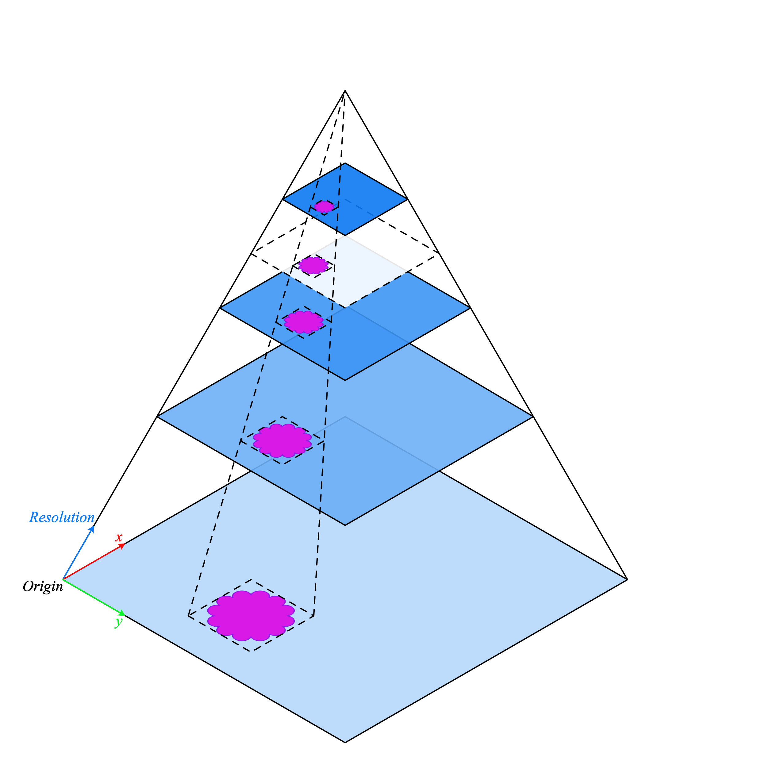 WSI 金字塔堆栈 (来源)
TIAToolbox 使我们能够自动化常见的下游分析任务,例如组织分类。在本教程中,我们将展示如何:1. 使用 TIAToolbox 加载 WSI 图像;以及 2. 使用不同的 PyTorch 模型在图像块级别对玻片进行分类。在本教程中,我们将提供一个使用 TorchVision 的 ResNet18 模型和自定义的 HistoEncoder <https://github.com/jopo666/HistoEncoder>`__ 模型的示例。
让我们开始吧!
设置环境
要运行本教程中提供的示例,需要以下软件包作为先决条件。
OpenJpeg
OpenSlide
Pixman
TIAToolbox
HistoEncoder(用于自定义模型示例)
请在您的终端中运行以下命令来安装这些软件包
apt-get -y -qq install libopenjp2-7-dev libopenjp2-tools openslide-tools libpixman-1-dev pip install -q ‘tiatoolbox<1.5’ histoencoder && echo “Installation is done.”
或者,您可以在 MacOS 上运行 brew install openjpeg openslide 来安装先决软件包,而不是使用 apt-get。有关安装的更多信息可以在此处找到。
运行前的清理
为确保适当清理(例如在异常终止时),本次运行中下载或创建的所有文件都保存在一个单独的目录 global_save_dir 中,我们将其设置为 “./tmp/”。为简化维护,目录名称仅在此处出现一次,以便在需要时轻松更改。
warnings.filterwarnings("ignore")
global_save_dir = Path("./tmp/")


def rmdir(dir_path: str | Path) -> None:
    """Helper function to delete directory."""
    if Path(dir_path).is_dir():
        shutil.rmtree(dir_path)
        logger.info("Removing directory %s", dir_path)


rmdir(global_save_dir)  # remove  directory if it exists from previous runs
global_save_dir.mkdir()
logger.info("Creating new directory %s", global_save_dir)
下载数据
对于我们的样本数据,我们将使用一张全玻片图像,以及来自 Kather 100k 数据集的验证子集的图像块。
wsi_path = global_save_dir / "sample_wsi.svs"
patches_path = global_save_dir / "kather100k-validation-sample.zip"
weights_path = global_save_dir / "resnet18-kather100k.pth"

logger.info("Download has started. Please wait...")

# Downloading and unzip a sample whole-slide image
download_data(
    "https://tiatoolbox.dcs.warwick.ac.uk/sample_wsis/TCGA-3L-AA1B-01Z-00-DX1.8923A151-A690-40B7-9E5A-FCBEDFC2394F.svs",
    wsi_path,
)

# Download and unzip a sample of the validation set used to train the Kather 100K dataset
download_data(
    "https://tiatoolbox.dcs.warwick.ac.uk/datasets/kather100k-validation-sample.zip",
    patches_path,
)
with ZipFile(patches_path, "r") as zipfile:
    zipfile.extractall(path=global_save_dir)

# Download pretrained model weights for WSI classification using ResNet18 architecture
download_data(
    "https://tiatoolbox.dcs.warwick.ac.uk/models/pc/resnet18-kather100k.pth",
    weights_path,
)

logger.info("Download is complete.")
读取数据
我们创建一个图像块列表和一个相应的标签列表。例如,label_list 中的第一个标签将指示 patch_list 中第一个图像块的类别。
# Read the patch data and create a list of patches and a list of corresponding labels
dataset_path = global_save_dir / "kather100k-validation-sample"
# Set the path to the dataset
image_ext = ".tif" # file extension of each image
# Obtain the mapping between the label ID and the class name
label_dict = {
"BACK": 0, # Background (empty glass region)
"NORM": 1, # Normal colon mucosa
"DEB": 2, # Debris
"TUM": 3, # Colorectal adenocarcinoma epithelium
"ADI": 4, # Adipose
"MUC": 5, # Mucus
"MUS": 6, # Smooth muscle
"STR": 7, # Cancer-associated stroma
"LYM": 8, # Lymphocytes
}
class_names = list(label_dict.keys())
class_labels = list(label_dict.values())
# Generate a list of patches and generate the label from the filename
patch_list = []
label_list = []
for class_name, label in label_dict.items():
dataset_class_path = dataset_path / class_name
patch_list_single_class = grab_files_from_dir(
dataset_class_path,
file_types="*" + image_ext,
)
patch_list.extend(patch_list_single_class)
label_list.extend([label] * len(patch_list_single_class))
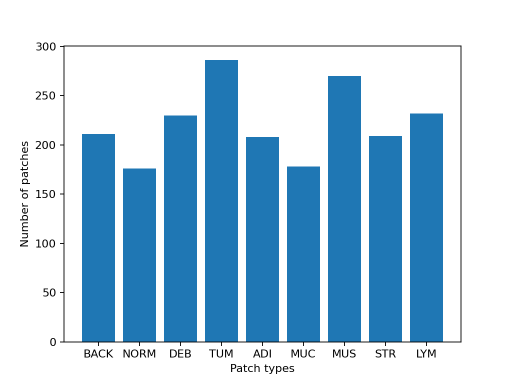
# Show some dataset statistics
plt.bar(class_names, [label_list.count(label) for label in class_labels])
plt.xlabel("Patch types")
plt.ylabel("Number of patches")
# Count the number of examples per class
for class_name, label in label_dict.items():
logger.info(
"Class ID: %d -- Class Name: %s -- Number of images: %d",
label,
class_name,
label_list.count(label),
)
# Overall dataset statistics
logger.info("Total number of patches: %d", (len(patch_list)))
|2023-11-14|13:15:59.299| [INFO] Class ID: 0 -- Class Name: BACK -- Number of images: 211
|2023-11-14|13:15:59.299| [INFO] Class ID: 1 -- Class Name: NORM -- Number of images: 176
|2023-11-14|13:15:59.299| [INFO] Class ID: 2 -- Class Name: DEB -- Number of images: 230
|2023-11-14|13:15:59.299| [INFO] Class ID: 3 -- Class Name: TUM -- Number of images: 286
|2023-11-14|13:15:59.299| [INFO] Class ID: 4 -- Class Name: ADI -- Number of images: 208
|2023-11-14|13:15:59.299| [INFO] Class ID: 5 -- Class Name: MUC -- Number of images: 178
|2023-11-14|13:15:59.299| [INFO] Class ID: 6 -- Class Name: MUS -- Number of images: 270
|2023-11-14|13:15:59.299| [INFO] Class ID: 7 -- Class Name: STR -- Number of images: 209
|2023-11-14|13:15:59.299| [INFO] Class ID: 8 -- Class Name: LYM -- Number of images: 232
|2023-11-14|13:15:59.299| [INFO] Total number of patches: 2000
正如您所见,对于这个图像块数据集,我们有 9 个类别/标签,ID 为 0-8,以及相关的类别名称,描述了图像块中的主要组织类型
BACK ⟶ 背景(空的玻片区域)
LYM ⟶ 淋巴细胞
NORM ⟶ 正常结肠黏膜
DEB ⟶ 碎屑
MUS ⟶ 平滑肌
STR ⟶ 癌症相关间质
ADI ⟶ 脂肪
MUC ⟶ 黏液
TUM ⟶ 结直肠腺癌上皮
对图像块进行分类
我们首先展示如何使用 patch 模式获取数字玻片中每个图像块的预测结果,然后使用 wsi 模式处理大型玻片。
定义 PatchPredictor 模型
PatchPredictor 类运行一个基于 CNN 的分类器,该分类器用 PyTorch 编写。
model可以是任何已训练的 PyTorch 模型,但有一个约束是它必须遵循tiatoolbox.models.abc.ModelABC(文档) <https://tia-toolbox.readthedocs.io/en/latest/_autosummary/tiatoolbox.models.models_abc.ModelABC.html>`__ 类结构。有关此事项的更多信息,请参阅我们关于高级模型技术的示例 notebook。为了加载自定义模型,您需要编写一个小型的预处理函数,如preproc_func(img)所示,它确保输入张量对于加载的网络来说格式正确。或者,您可以将
pretrained_model作为字符串参数传递。这指定了执行预测的 CNN 模型,并且它必须是此处列出的模型之一。命令将如下所示:predictor = PatchPredictor(pretrained_model='resnet18-kather100k', pretrained_weights=weights_path, batch_size=32)。pretrained_weights:使用pretrained_model时,默认也会下载相应的预训练权重。您可以通过pretrained_weight参数使用自己的权重集来覆盖默认设置。batch_size:每次馈送给模型的图像数量。此参数的值越大,需要更大的 (GPU) 内存容量。
# Importing a pretrained PyTorch model from TIAToolbox
predictor = PatchPredictor(pretrained_model='resnet18-kather100k', batch_size=32)

# Users can load any PyTorch model architecture instead using the following script
model = vanilla.CNNModel(backbone="resnet18", num_classes=9) # Importing model from torchvision.models.resnet18
model.load_state_dict(torch.load(weights_path, map_location="cpu", weights_only=True), strict=True)
def preproc_func(img):
    img = PIL.Image.fromarray(img)
    img = transforms.ToTensor()(img)
    return img.permute(1, 2, 0)
model.preproc_func = preproc_func
predictor = PatchPredictor(model=model, batch_size=32)
预测图像块标签
我们创建一个预测器对象,然后使用 patch 模式调用 predict 方法。然后我们计算分类精度和混淆矩阵。
with suppress_console_output():
    output = predictor.predict(imgs=patch_list, mode="patch", on_gpu=ON_GPU)

acc = accuracy_score(label_list, output["predictions"])
logger.info("Classification accuracy: %f", acc)

# Creating and visualizing the confusion matrix for patch classification results
conf = confusion_matrix(label_list, output["predictions"], normalize="true")
df_cm = pd.DataFrame(conf, index=class_names, columns=class_names)
df_cm
|2023-11-14|13:16:03.215| [INFO] Classification accuracy: 0.993000
预测全玻片图像块标签
现在我们介绍 IOPatchPredictorConfig,这是一个类,用于指定模型预测引擎的图像读取和预测写入配置。这是必需的,以便告知分类器应读取 WSI 金字塔的哪个级别,处理数据并生成输出。
IOPatchPredictorConfig 的参数定义如下
input_resolutions:一个列表,以字典形式指定每个输入的解析度。列表元素必须与目标model.forward()中的顺序相同。如果您的模型只接受一个输入,您只需放入一个字典指定'units'和'resolution'。请注意,TIAToolbox 支持具有多个输入的模型。有关单位和解析度的更多信息,请参阅 TIAToolbox 文档。patch_input_shape:最大输入图像的形状,格式为 (高度, 宽度)。stride_shape:用于图像块提取过程中,两个连续图像块之间的步长大小。如果用户将stride_shape设置为等于patch_input_shape,则提取和处理的图像块将没有任何重叠。
wsi_ioconfig = IOPatchPredictorConfig(
    input_resolutions=[{"units": "mpp", "resolution": 0.5}],
    patch_input_shape=[224, 224],
    stride_shape=[224, 224],
)
predict 方法将 CNN 应用于输入图像块并获取结果。以下是参数及其说明
mode:要处理的输入类型。根据您的应用选择patch、tile或wsi。imgs:输入列表,应为输入 tile 或 WSI 的路径列表。return_probabilities:设置为 True 以获取每个图像块的预测标签以及各类别概率。如果您希望合并预测结果以生成tile或wsi模式下的预测图,可以将return_probabilities设置为 True。ioconfig:使用IOPatchPredictorConfig类设置 IO 配置信息。resolution和unit(未在下面显示):这些参数指定了我们计划从中提取图像块的 WSI 级别的级别或每像素微米分辨率,并且可以用来代替ioconfig。在此,我们将 WSI 级别指定为'baseline',这相当于级别 0。通常,这是分辨率最高的级别。在本例中,图像只有一个级别。更多信息请参见文档。masks:与imgs列表中 WSI 掩膜对应的路径列表。这些掩膜指定了我们想要从中提取图像块的原始 WSI 中的区域。如果某个 WSI 的掩膜指定为None,则将预测该 WSI 所有图像块(甚至包括背景区域)的标签。这可能会导致不必要的计算。merge_predictions:如果需要生成图像块分类结果的 2D 图,您可以将此参数设置为True。然而,对于大型 WSI,这将需要大量可用内存。另一种(默认)解决方案是将merge_predictions设置为False,然后使用merge_predictions函数生成 2D 预测图,正如您稍后将看到的那样。
由于我们使用的是大型 WSI,图像块提取和预测过程可能需要一些时间(如果您有支持 Cuda 的 GPU 并已安装 PyTorch+Cuda,请确保将 ON_GPU 设置为 True)。
with suppress_console_output():
    wsi_output = predictor.predict(
        imgs=[wsi_path],
        masks=None,
        mode="wsi",
        merge_predictions=False,
        ioconfig=wsi_ioconfig,
        return_probabilities=True,
        save_dir=global_save_dir / "wsi_predictions",
        on_gpu=ON_GPU,
    )
通过可视化 wsi_output,我们可以看到预测模型在我们的全玻片图像上的工作情况。我们首先需要合并图像块预测输出,然后将其作为叠加层可视化到原始图像上。像之前一样,使用 merge_predictions 方法来合并图像块预测结果。此处,我们将参数 resolution=1.25, units='power' 设置为在 1.25 倍放大倍率下生成预测图。如果您希望获得更高/更低分辨率(更大/更小)的预测图,您需要相应地更改这些参数。预测结果合并后,使用 overlay_patch_prediction 函数将预测图叠加在 WSI 缩略图上,缩略图应以用于预测合并的分辨率提取。
overview_resolution = (
    4  # the resolution in which we desire to merge and visualize the patch predictions
)
# the unit of the `resolution` parameter. Can be "power", "level", "mpp", or "baseline"
overview_unit = "mpp"
wsi = WSIReader.open(wsi_path)
wsi_overview = wsi.slide_thumbnail(resolution=overview_resolution, units=overview_unit)
plt.figure(), plt.imshow(wsi_overview)
plt.axis("off")
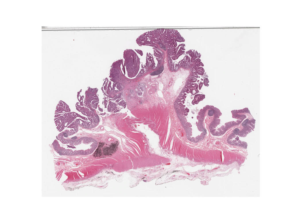
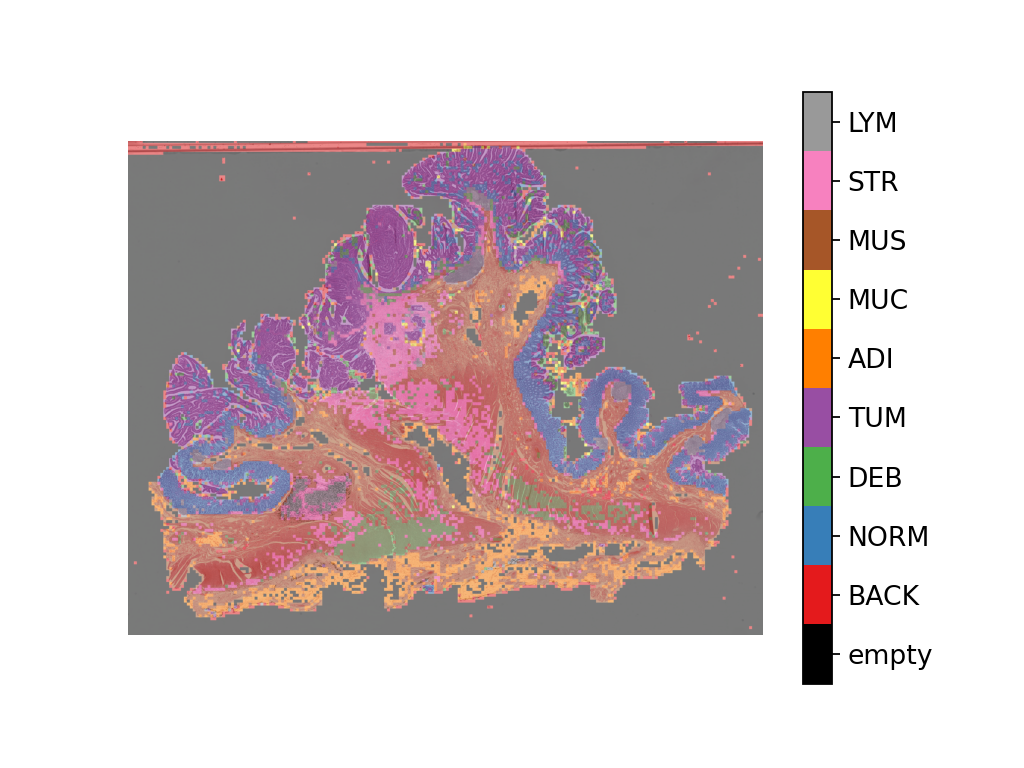
将预测图叠加在此图像上,结果如下所示
# Visualization of whole-slide image patch-level prediction
# first set up a label to color mapping
label_color_dict = {}
label_color_dict[0] = ("empty", (0, 0, 0))
colors = cm.get_cmap("Set1").colors
for class_name, label in label_dict.items():
    label_color_dict[label + 1] = (class_name, 255 * np.array(colors[label]))

pred_map = predictor.merge_predictions(
    wsi_path,
    wsi_output[0],
    resolution=overview_resolution,
    units=overview_unit,
)
overlay = overlay_prediction_mask(
    wsi_overview,
    pred_map,
    alpha=0.5,
    label_info=label_color_dict,
    return_ax=True,
)
plt.show()
使用病理学专用模型进行特征提取
在本节中,我们将展示如何使用 TIAToolbox 提供的 WSI 推理引擎,从 TIAToolbox 外部存在的预训练 PyTorch 模型中提取特征。为了说明这一点,我们将使用 HistoEncoder,这是一个计算病理学专用模型,该模型以自监督方式训练,用于从组织病理学图像中提取特征。该模型已在此处提供
由赫尔辛基大学的 Pohjonen, Joona 及其团队提供的“HistoEncoder:数字病理学基础模型”(https://github.com/jopo666/HistoEncoder)。
我们将绘制特征图的 umap 降维到 3D (RGB),以可视化这些特征如何捕捉上述某些组织类型之间的差异。
# Import some extra modules
import histoencoder.functional as F
import torch.nn as nn

from tiatoolbox.models.engine.semantic_segmentor import DeepFeatureExtractor, IOSegmentorConfig
from tiatoolbox.models.models_abc import ModelABC
import umap
TIAToolbox 定义了一个 ModelABC,这是一个继承自 PyTorch nn.Module 的类,并指定了模型为了在 TIAToolbox 推理引擎中使用应该具备的结构。histoencoder 模型不遵循此结构,因此我们需要将其包装在一个类中,该类的输出和方法是 TIAToolbox 引擎所期望的。
class HistoEncWrapper(ModelABC):
    """Wrapper for HistoEnc model that conforms to tiatoolbox ModelABC interface."""

    def __init__(self: HistoEncWrapper, encoder) -> None:
        super().__init__()
        self.feat_extract = encoder

    def forward(self: HistoEncWrapper, imgs: torch.Tensor) -> torch.Tensor:
        """Pass input data through the model.

        Args:
            imgs (torch.Tensor):
                Model input.

        """
        out = F.extract_features(self.feat_extract, imgs, num_blocks=2, avg_pool=True)
        return out

    @staticmethod
    def infer_batch(
        model: nn.Module,
        batch_data: torch.Tensor,
        *,
        on_gpu: bool,
    ) -> list[np.ndarray]:
        """Run inference on an input batch.

        Contains logic for forward operation as well as i/o aggregation.

        Args:
            model (nn.Module):
                PyTorch defined model.
            batch_data (torch.Tensor):
                A batch of data generated by
                `torch.utils.data.DataLoader`.
            on_gpu (bool):
                Whether to run inference on a GPU.

        """
        img_patches_device = batch_data.to('cuda') if on_gpu else batch_data
        model.eval()
        # Do not compute the gradient (not training)
        with torch.inference_mode():
            output = model(img_patches_device)
        return [output.cpu().numpy()]
现在我们有了包装器,我们将创建我们的特征提取模型,并实例化一个 DeepFeatureExtractor,以便我们可以在 WSI 上使用此模型。我们将使用上面相同的 WSI,但这次我们将使用 HistoEncoder 模型从 WSI 的图像块中提取特征,而不是预测每个图像块的某个标签。
# create the model
encoder = F.create_encoder("prostate_medium")
model = HistoEncWrapper(encoder)

# set the pre-processing function
norm=transforms.Normalize(mean=[0.662, 0.446, 0.605],std=[0.169, 0.190, 0.155])
trans = [
    transforms.ToTensor(),
    norm,
]
model.preproc_func = transforms.Compose(trans)

wsi_ioconfig = IOSegmentorConfig(
    input_resolutions=[{"units": "mpp", "resolution": 0.5}],
    patch_input_shape=[224, 224],
    output_resolutions=[{"units": "mpp", "resolution": 0.5}],
    patch_output_shape=[224, 224],
    stride_shape=[224, 224],
)
当我们创建 DeepFeatureExtractor 时,我们将传递 auto_generate_mask=True 参数。这将使用 otsu 阈值自动创建组织区域的掩膜,以便提取器只处理包含组织的图像块。
# create the feature extractor and run it on the WSI
extractor = DeepFeatureExtractor(model=model, auto_generate_mask=True, batch_size=32, num_loader_workers=4, num_postproc_workers=4)
with suppress_console_output():
    out = extractor.predict(imgs=[wsi_path], mode="wsi", ioconfig=wsi_ioconfig, save_dir=global_save_dir / "wsi_features",)
这些特征可用于训练下游模型,但在此处,为了了解这些特征代表什么,我们将使用 UMAP 降维在 RGB 空间中可视化特征。颜色相似的点应该具有相似的特征,因此我们可以检查当我们将 UMAP 降维结果叠加到 WSI 缩略图上时,特征是否会自然地分离到不同的组织区域。我们将在下面的单元格中将其与上面的图像块级预测图一起绘制,以查看特征与图像块级预测结果的比较情况。
# First we define a function to calculate the umap reduction
def umap_reducer(x, dims=3, nns=10):
    """UMAP reduction of the input data."""
    reducer = umap.UMAP(n_neighbors=nns, n_components=dims, metric="manhattan", spread=0.5, random_state=2)
    reduced = reducer.fit_transform(x)
    reduced -= reduced.min(axis=0)
    reduced /= reduced.max(axis=0)
    return reduced

# load the features output by our feature extractor
pos = np.load(global_save_dir / "wsi_features" / "0.position.npy")
feats = np.load(global_save_dir / "wsi_features" / "0.features.0.npy")
pos = pos / 8 # as we extracted at 0.5mpp, and we are overlaying on a thumbnail at 4mpp

# reduce the features into 3 dimensional (rgb) space
reduced = umap_reducer(feats)

# plot the prediction map the classifier again
overlay = overlay_prediction_mask(
    wsi_overview,
    pred_map,
    alpha=0.5,
    label_info=label_color_dict,
    return_ax=True,
)

# plot the feature map reduction
plt.figure()
plt.imshow(wsi_overview)
plt.scatter(pos[:,0], pos[:,1], c=reduced, s=1, alpha=0.5)
plt.axis("off")
plt.title("UMAP reduction of HistoEnc features")
plt.show()

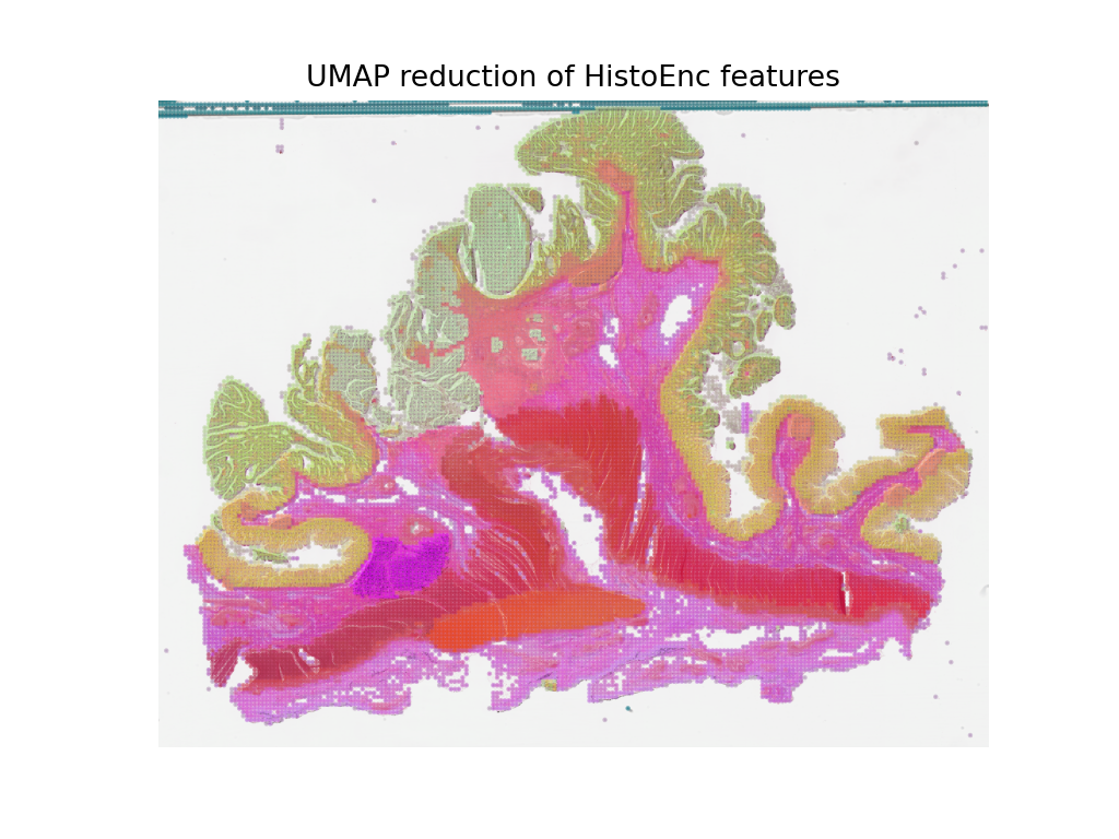
我们看到,来自我们的图像块级预测器的预测图,以及来自我们的自监督特征编码器的特征图,捕捉了关于 WSI 中组织类型的相似信息。这是一个很好的健全性检查,表明我们的模型按预期工作。这也表明,HistoEncoder 模型提取的特征捕捉了组织类型之间的差异,因此它们编码了与组织学相关的信息。
后续步骤
在本 notebook 中,我们展示了如何使用 PatchPredictor 和 DeepFeatureExtractor 类及其 predict 方法来预测大型 tile 和 WSI 的图像块的标签,或提取特征。我们介绍了 merge_predictions 和 overlay_prediction_mask 辅助函数,这些函数合并图像块预测输出,并将结果预测图可视化为输入图像/WSI 上的叠加层。
所有过程都在 TIAToolbox 内部进行,我们可以按照我们的示例代码轻松地将各部分组合起来。请确保正确设置输入和选项。我们鼓励您进一步研究更改 predict 函数参数对预测输出的影响。我们已经演示了如何使用您自己的预训练模型或研究社区提供的特定任务模型在 TIAToolbox 框架中对大型 WSI 进行推理,即使模型结构未在 TIAToolbox 模型类中定义。
您可以通过以下资源了解更多信息
