注意

点击此处下载完整示例代码

PyTorch 数字套件教程¶

创建于: 2020 年 7 月 28 日 | 最后更新: 2024 年 1 月 16 日 | 最后验证: 未验证

引言¶

量化在奏效时效果很好，但当其无法满足我们预期的精度时，就很难知道问题出在哪里。调试量化精度问题并非易事且耗时。

调试的一个重要步骤是测量浮点模型及其对应量化模型的统计数据，以了解它们在哪方面差异最大。我们在 PyTorch 量化中构建了一套称为 PyTorch Numeric Suite 的数字工具，用于测量量化模块和浮点模块之间的统计数据，以支持量化调试工作。即使对于精度良好的量化模型，PyTorch Numeric Suite 仍然可以用作性能分析工具，以更好地理解模型中的量化误差，并为进一步优化提供指导。

PyTorch Numeric Suite 目前支持通过静态量化和动态量化获得的模型，并提供统一的 API。

在本教程中，我们将首先使用 ResNet18 作为示例，演示如何使用 PyTorch Numeric Suite 在 eager 模式下测量静态量化模型和浮点模型之间的统计数据。然后，我们将使用基于 LSTM 的序列模型作为示例，演示 PyTorch Numeric Suite 在动态量化模型中的用法。

静态量化的数字套件¶

设置¶

我们将首先进行必要的导入

import numpy as np
import torch
import torch.nn as nn
import torchvision
from torchvision import models, datasets
import torchvision.transforms as transforms
import os
import torch.quantization
import torch.quantization._numeric_suite as ns
from torch.quantization import (
    default_eval_fn,
    default_qconfig,
    quantize,
)

然后我们加载预训练的浮点 ResNet18 模型，并将其量化为 qmodel。我们不能比较任意两个模型，只能比较一个浮点模型及其派生的量化模型。

float_model = torchvision.models.quantization.resnet18(weights=models.ResNet18_Weights.IMAGENET1K_V1, quantize=False)
float_model.to('cpu')
float_model.eval()
float_model.fuse_model()
float_model.qconfig = torch.quantization.default_qconfig
img_data = [(torch.rand(2, 3, 10, 10, dtype=torch.float), torch.randint(0, 1, (2,), dtype=torch.long)) for _ in range(2)]
qmodel = quantize(float_model, default_eval_fn, [img_data], inplace=False)

1. 比较浮点模型和量化模型的权重¶

我们通常首先要比较的是量化模型和浮点模型的权重。我们可以调用 PyTorch Numeric Suite 中的 compare_weights() 函数，以获取一个字典 wt_compare_dict，其键对应于模块名称，每个条目是一个包含‘float’和‘quantized’两个键的字典，分别包含浮点和量化的权重。compare_weights() 接收浮点和量化模型的 state dict，并返回一个字典，其键对应于浮点权重，值是一个包含浮点和量化权重的字典

wt_compare_dict = ns.compare_weights(float_model.state_dict(), qmodel.state_dict())

print('keys of wt_compare_dict:')
print(wt_compare_dict.keys())

print("\nkeys of wt_compare_dict entry for conv1's weight:")
print(wt_compare_dict['conv1.weight'].keys())
print(wt_compare_dict['conv1.weight']['float'].shape)
print(wt_compare_dict['conv1.weight']['quantized'].shape)

keys of wt_compare_dict:
dict_keys(['conv1.weight', 'layer1.0.conv1.weight', 'layer1.0.conv2.weight', 'layer1.1.conv1.weight', 'layer1.1.conv2.weight', 'layer2.0.conv1.weight', 'layer2.0.conv2.weight', 'layer2.0.downsample.0.weight', 'layer2.1.conv1.weight', 'layer2.1.conv2.weight', 'layer3.0.conv1.weight', 'layer3.0.conv2.weight', 'layer3.0.downsample.0.weight', 'layer3.1.conv1.weight', 'layer3.1.conv2.weight', 'layer4.0.conv1.weight', 'layer4.0.conv2.weight', 'layer4.0.downsample.0.weight', 'layer4.1.conv1.weight', 'layer4.1.conv2.weight', 'fc._packed_params._packed_params'])

keys of wt_compare_dict entry for conv1's weight:
dict_keys(['float', 'quantized'])
torch.Size([64, 3, 7, 7])
torch.Size([64, 3, 7, 7])

获取 wt_compare_dict 后，用户可以按照他们想要的方式处理这个字典。这里作为示例，我们计算浮点模型和量化模型权重的量化误差如下。计算量化张量 y 的信噪比 (SQNR)。SQNR 反映了最大标称信号强度与量化过程中引入的量化误差之间的关系。SQNR 越高，对应的量化误差越低。

def compute_error(x, y):
    Ps = torch.norm(x)
    Pn = torch.norm(x-y)
    return 20*torch.log10(Ps/Pn)

for key in wt_compare_dict:
    print(key, compute_error(wt_compare_dict[key]['float'], wt_compare_dict[key]['quantized'].dequantize()))

conv1.weight tensor(31.6638)
layer1.0.conv1.weight tensor(30.6450)
layer1.0.conv2.weight tensor(31.1528)
layer1.1.conv1.weight tensor(32.1438)
layer1.1.conv2.weight tensor(31.2477)
layer2.0.conv1.weight tensor(30.9890)
layer2.0.conv2.weight tensor(28.8233)
layer2.0.downsample.0.weight tensor(31.5558)
layer2.1.conv1.weight tensor(30.7668)
layer2.1.conv2.weight tensor(28.4516)
layer3.0.conv1.weight tensor(30.9247)
layer3.0.conv2.weight tensor(26.6841)
layer3.0.downsample.0.weight tensor(28.7825)
layer3.1.conv1.weight tensor(28.9707)
layer3.1.conv2.weight tensor(25.6784)
layer4.0.conv1.weight tensor(26.8495)
layer4.0.conv2.weight tensor(25.8394)
layer4.0.downsample.0.weight tensor(28.6355)
layer4.1.conv1.weight tensor(26.8758)
layer4.1.conv2.weight tensor(28.4319)
fc._packed_params._packed_params tensor(32.6505)

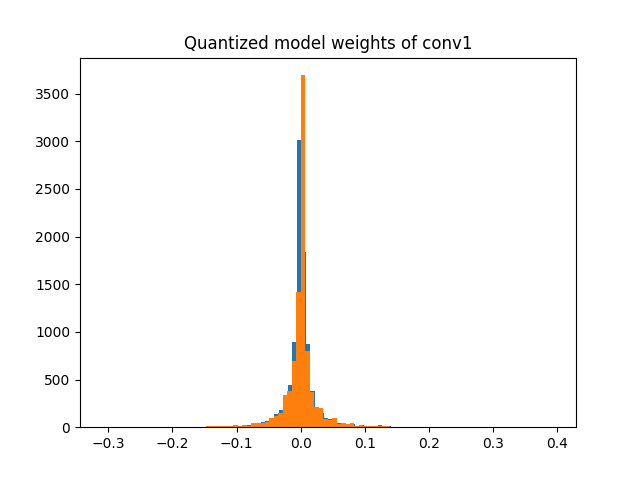
作为另一个示例，wt_compare_dict 也可以用来绘制浮点模型和量化模型权重的直方图。

import matplotlib.pyplot as plt

f = wt_compare_dict['conv1.weight']['float'].flatten()
plt.hist(f, bins = 100)
plt.title("Floating point model weights of conv1")
plt.show()

q = wt_compare_dict['conv1.weight']['quantized'].flatten().dequantize()
plt.hist(q, bins = 100)
plt.title("Quantized model weights of conv1")
plt.show()

2. 在对应位置比较浮点模型和量化模型¶

第二个工具允许在对应位置比较浮点模型和量化模型的权重和激活，输入数据相同，如下图所示。红色箭头表示比较的位置。

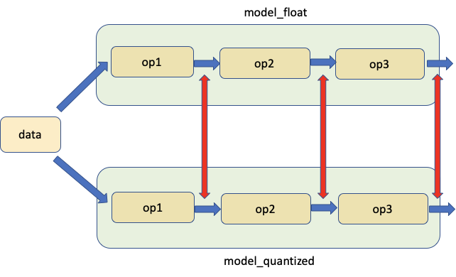
我们调用 PyTorch Numeric Suite 中的 compare_model_outputs() 函数，以获取浮点模型和量化模型在给定输入数据对应位置的激活。这个 API 返回一个字典，键是模块名称。每个条目本身是一个包含‘float’和‘quantized’两个键的字典，包含激活。

data = img_data[0][0]

# Take in floating point and quantized model as well as input data, and returns a dict, with keys
# corresponding to the quantized module names and each entry being a dictionary with two keys 'float' and
# 'quantized', containing the activations of floating point and quantized model at matching locations.
act_compare_dict = ns.compare_model_outputs(float_model, qmodel, data)

print('keys of act_compare_dict:')
print(act_compare_dict.keys())

print("\nkeys of act_compare_dict entry for conv1's output:")
print(act_compare_dict['conv1.stats'].keys())
print(act_compare_dict['conv1.stats']['float'][0].shape)
print(act_compare_dict['conv1.stats']['quantized'][0].shape)

keys of act_compare_dict:
dict_keys(['conv1.stats', 'layer1.0.conv1.stats', 'layer1.0.conv2.stats', 'layer1.0.add_relu.stats', 'layer1.1.conv1.stats', 'layer1.1.conv2.stats', 'layer1.1.add_relu.stats', 'layer2.0.conv1.stats', 'layer2.0.conv2.stats', 'layer2.0.downsample.0.stats', 'layer2.0.add_relu.stats', 'layer2.1.conv1.stats', 'layer2.1.conv2.stats', 'layer2.1.add_relu.stats', 'layer3.0.conv1.stats', 'layer3.0.conv2.stats', 'layer3.0.downsample.0.stats', 'layer3.0.add_relu.stats', 'layer3.1.conv1.stats', 'layer3.1.conv2.stats', 'layer3.1.add_relu.stats', 'layer4.0.conv1.stats', 'layer4.0.conv2.stats', 'layer4.0.downsample.0.stats', 'layer4.0.add_relu.stats', 'layer4.1.conv1.stats', 'layer4.1.conv2.stats', 'layer4.1.add_relu.stats', 'fc.stats', 'quant.stats'])

keys of act_compare_dict entry for conv1's output:
dict_keys(['float', 'quantized'])
torch.Size([2, 64, 5, 5])
torch.Size([2, 64, 5, 5])

这个字典可以用来比较和计算浮点模型和量化模型激活的量化误差如下。

for key in act_compare_dict:
    print(key, compute_error(act_compare_dict[key]['float'][0], act_compare_dict[key]['quantized'][0].dequantize()))

conv1.stats tensor(37.1388, grad_fn=<MulBackward0>)
layer1.0.conv1.stats tensor(30.1562, grad_fn=<MulBackward0>)
layer1.0.conv2.stats tensor(29.0511, grad_fn=<MulBackward0>)
layer1.0.add_relu.stats tensor(32.7605, grad_fn=<MulBackward0>)
layer1.1.conv1.stats tensor(30.1330, grad_fn=<MulBackward0>)
layer1.1.conv2.stats tensor(26.3872, grad_fn=<MulBackward0>)
layer1.1.add_relu.stats tensor(30.0649, grad_fn=<MulBackward0>)
layer2.0.conv1.stats tensor(26.9528, grad_fn=<MulBackward0>)
layer2.0.conv2.stats tensor(26.7812, grad_fn=<MulBackward0>)
layer2.0.downsample.0.stats tensor(23.2544, grad_fn=<MulBackward0>)
layer2.0.add_relu.stats tensor(26.2048, grad_fn=<MulBackward0>)
layer2.1.conv1.stats tensor(25.6735, grad_fn=<MulBackward0>)
layer2.1.conv2.stats tensor(24.6564, grad_fn=<MulBackward0>)
layer2.1.add_relu.stats tensor(26.0816, grad_fn=<MulBackward0>)
layer3.0.conv1.stats tensor(26.9846, grad_fn=<MulBackward0>)
layer3.0.conv2.stats tensor(26.8694, grad_fn=<MulBackward0>)
layer3.0.downsample.0.stats tensor(25.1453, grad_fn=<MulBackward0>)
layer3.0.add_relu.stats tensor(24.8748, grad_fn=<MulBackward0>)
layer3.1.conv1.stats tensor(31.0022, grad_fn=<MulBackward0>)
layer3.1.conv2.stats tensor(26.1478, grad_fn=<MulBackward0>)
layer3.1.add_relu.stats tensor(25.5775, grad_fn=<MulBackward0>)
layer4.0.conv1.stats tensor(27.4940, grad_fn=<MulBackward0>)
layer4.0.conv2.stats tensor(27.2149, grad_fn=<MulBackward0>)
layer4.0.downsample.0.stats tensor(22.5105, grad_fn=<MulBackward0>)
layer4.0.add_relu.stats tensor(21.2105, grad_fn=<MulBackward0>)
layer4.1.conv1.stats tensor(26.5055, grad_fn=<MulBackward0>)
layer4.1.conv2.stats tensor(18.5702, grad_fn=<MulBackward0>)
layer4.1.add_relu.stats tensor(18.5091, grad_fn=<MulBackward0>)
fc.stats tensor(20.7117, grad_fn=<MulBackward0>)
quant.stats tensor(47.9043)

如果我们要对多个输入数据进行比较，可以执行以下操作。如果模块在 white_list 中，则通过将 logger 附加到浮点模块和量化模块来准备模型。默认 logger 是 OutputLogger，默认 white_list 是 DEFAULT_NUMERIC_SUITE_COMPARE_MODEL_OUTPUT_WHITE_LIST

ns.prepare_model_outputs(float_model, qmodel)

for data in img_data:
    float_model(data[0])
    qmodel(data[0])

# Find the matching activation between floating point and quantized modules, and return a dict with key
# corresponding to quantized module names and each entry being a dictionary with two keys 'float'
# and 'quantized', containing the matching floating point and quantized activations logged by the logger
act_compare_dict = ns.get_matching_activations(float_model, qmodel)

上述 API 中使用的默认 logger 是 OutputLogger，它用于记录模块的输出。我们可以继承基础 Logger 类并创建我们自己的 logger 来执行不同的功能。例如，我们可以创建一个新的 MyOutputLogger 类如下。

class MyOutputLogger(ns.Logger):
    r"""Customized logger class
    """

    def __init__(self):
        super(MyOutputLogger, self).__init__()

    def forward(self, x):
        # Custom functionalities
        # ...
        return x

然后我们可以将此 logger 传递给上述 API，例如

data = img_data[0][0]
act_compare_dict = ns.compare_model_outputs(float_model, qmodel, data, logger_cls=MyOutputLogger)

或

ns.prepare_model_outputs(float_model, qmodel, MyOutputLogger)
for data in img_data:
    float_model(data[0])
    qmodel(data[0])
act_compare_dict = ns.get_matching_activations(float_model, qmodel)

3. 使用相同输入数据比较量化模型中的模块及其对应的浮点模块¶

第三个工具允许将模型中的量化模块与其对应的浮点模块进行比较，两者输入相同数据，并比较它们的输出，如下图所示。

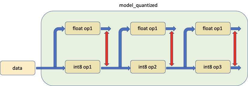
在实践中，我们调用 prepare_model_with_stubs() 来将我们要比较的量化模块与 Shadow 模块进行替换，如下所示

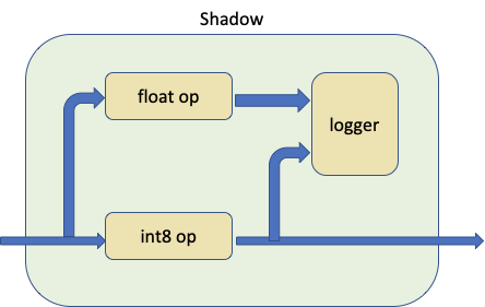
Shadow 模块将量化模块、浮点模块和 logger 作为输入，并在内部创建一个前向路径，使浮点模块跟随量化模块，共享相同的输入张量。

logger 可以自定义，默认 logger 是 ShadowLogger，它将保存量化模块和浮点模块的输出，可用于计算模块级别的量化误差。

请注意，在每次调用 compare_model_outputs() 和 compare_model_stub() 之前，我们需要有干净的浮点模型和量化模型。这是因为 compare_model_outputs() 和 compare_model_stub() 会就地修改浮点模型和量化模型，如果连续调用，将导致意外结果。

float_model = torchvision.models.quantization.resnet18(weights=models.ResNet18_Weights.IMAGENET1K_V1, quantize=False)
float_model.to('cpu')
float_model.eval()
float_model.fuse_model()
float_model.qconfig = torch.quantization.default_qconfig
img_data = [(torch.rand(2, 3, 10, 10, dtype=torch.float), torch.randint(0, 1, (2,), dtype=torch.long)) for _ in range(2)]
qmodel = quantize(float_model, default_eval_fn, [img_data], inplace=False)

在下面的示例中，我们调用 PyTorch Numeric Suite 中的 compare_model_stub() 函数，以比较 QuantizableBasicBlock 模块与其对应的浮点模块。这个 API 返回一个字典，其键对应于模块名称，每个条目是一个包含‘float’和‘quantized’两个键的字典，包含量化模块及其匹配的浮点 Shadow 模块的输出张量。

data = img_data[0][0]
module_swap_list = [torchvision.models.quantization.resnet.QuantizableBasicBlock]

# Takes in floating point and quantized model as well as input data, and returns a dict with key
# corresponding to module names and each entry being a dictionary with two keys 'float' and
# 'quantized', containing the output tensors of quantized module and its matching floating point shadow module.
ob_dict = ns.compare_model_stub(float_model, qmodel, module_swap_list, data)

print('keys of ob_dict:')
print(ob_dict.keys())

print("\nkeys of ob_dict entry for layer1.0's output:")
print(ob_dict['layer1.0.stats'].keys())
print(ob_dict['layer1.0.stats']['float'][0].shape)
print(ob_dict['layer1.0.stats']['quantized'][0].shape)

keys of ob_dict:
dict_keys(['layer1.0.stats', 'layer1.1.stats', 'layer2.0.stats', 'layer2.1.stats', 'layer3.0.stats', 'layer3.1.stats', 'layer4.0.stats', 'layer4.1.stats'])

keys of ob_dict entry for layer1.0's output:
dict_keys(['float', 'quantized'])
torch.Size([64, 3, 3])
torch.Size([64, 3, 3])

然后可以使用这个字典来比较和计算模块级别的量化误差。

for key in ob_dict:
    print(key, compute_error(ob_dict[key]['float'][0], ob_dict[key]['quantized'][0].dequantize()))

layer1.0.stats tensor(32.7203)
layer1.1.stats tensor(34.8070)
layer2.0.stats tensor(29.3657)
layer2.1.stats tensor(31.0864)
layer3.0.stats tensor(28.5980)
layer3.1.stats tensor(31.3857)
layer4.0.stats tensor(25.3010)
layer4.1.stats tensor(22.9801)

如果我们要对多个输入数据进行比较，可以执行以下操作。

ns.prepare_model_with_stubs(float_model, qmodel, module_swap_list, ns.ShadowLogger)
for data in img_data:
    qmodel(data[0])
ob_dict = ns.get_logger_dict(qmodel)

上述 API 中使用的默认 logger 是 ShadowLogger，它用于记录量化模块及其匹配的浮点 Shadow 模块的输出。我们可以继承基础 Logger 类并创建我们自己的 logger 来执行不同的功能。例如，我们可以创建一个新的 MyShadowLogger 类如下。

class MyShadowLogger(ns.Logger):
    r"""Customized logger class
    """

    def __init__(self):
        super(MyShadowLogger, self).__init__()

    def forward(self, x, y):
        # Custom functionalities
        # ...
        return x

然后我们可以将此 logger 传递给上述 API，例如

data = img_data[0][0]
ob_dict = ns.compare_model_stub(float_model, qmodel, module_swap_list, data, logger_cls=MyShadowLogger)

或

ns.prepare_model_with_stubs(float_model, qmodel, module_swap_list, MyShadowLogger)
for data in img_data:
    qmodel(data[0])
ob_dict = ns.get_logger_dict(qmodel)

动态量化的数字套件¶

Numeric Suite API 的设计方式使其适用于动态量化模型和静态量化模型。我们将使用一个包含 LSTM 和 Linear 模块的模型来演示 Numeric Suite 在动态量化模型上的用法。该模型与 LSTM 词语言模型动态量化教程 [1] 中使用的模型相同。

设置¶

首先我们定义模型如下。请注意，在此模型中，只有 nn.LSTM 和 nn.Linear 模块将进行动态量化，而 nn.Embedding 在量化后仍将保持为浮点模块。

class LSTMModel(nn.Module):
    """Container module with an encoder, a recurrent module, and a decoder."""

    def __init__(self, ntoken, ninp, nhid, nlayers, dropout=0.5):
        super(LSTMModel, self).__init__()
        self.encoder = nn.Embedding(ntoken, ninp)
        self.rnn = nn.LSTM(ninp, nhid, nlayers, dropout=dropout)
        self.decoder = nn.Linear(nhid, ntoken)

        self.init_weights()

        self.nhid = nhid
        self.nlayers = nlayers

    def init_weights(self):
        initrange = 0.1
        self.encoder.weight.data.uniform_(-initrange, initrange)
        self.decoder.bias.data.zero_()
        self.decoder.weight.data.uniform_(-initrange, initrange)

    def forward(self, input, hidden):
        emb = self.encoder(input)
        output, hidden = self.rnn(emb, hidden)
        decoded = self.decoder(output)
        return decoded, hidden

    def init_hidden(self, bsz):
        weight = next(self.parameters())
        return (weight.new_zeros(self.nlayers, bsz, self.nhid),
                weight.new_zeros(self.nlayers, bsz, self.nhid))

然后我们创建 float_model 并将其量化为 qmodel。

ntokens = 10

float_model = LSTMModel(
    ntoken = ntokens,
    ninp = 512,
    nhid = 256,
    nlayers = 5,
)

float_model.eval()

qmodel = torch.quantization.quantize_dynamic(
    float_model, {nn.LSTM, nn.Linear}, dtype=torch.qint8
)

1. 比较浮点模型和量化模型的权重¶

我们首先调用 PyTorch Numeric Suite 中的 compare_weights() 函数，以获取一个字典 wt_compare_dict，其键对应于模块名称，每个条目是一个包含‘float’和‘quantized’两个键的字典，包含浮点和量化的权重。

wt_compare_dict = ns.compare_weights(float_model.state_dict(), qmodel.state_dict())

获取 wt_compare_dict 后，可以用来比较和计算浮点模型和量化模型权重的量化误差如下。

for key in wt_compare_dict:
    if wt_compare_dict[key]['quantized'].is_quantized:
        print(key, compute_error(wt_compare_dict[key]['float'], wt_compare_dict[key]['quantized'].dequantize()))
    else:
        print(key, compute_error(wt_compare_dict[key]['float'], wt_compare_dict[key]['quantized']))

encoder.weight tensor(inf)
rnn._all_weight_values.0.param tensor(48.1323)
rnn._all_weight_values.1.param tensor(48.1355)
rnn._all_weight_values.2.param tensor(48.1213)
rnn._all_weight_values.3.param tensor(48.1506)
rnn._all_weight_values.4.param tensor(48.1348)
decoder._packed_params._packed_params tensor(48.0233)

上面 encoder.weight 条目中的 Inf 值是因为 encoder 模块未量化，其权重在浮点模型和量化模型中是相同的。

2. 在对应位置比较浮点模型和量化模型¶

然后我们调用 PyTorch Numeric Suite 中的 compare_model_outputs() 函数，以获取浮点模型和量化模型在给定输入数据对应位置的激活。这个 API 返回一个字典，键是模块名称。每个条目本身是一个包含‘float’和‘quantized’两个键的字典，包含激活。请注意，这个序列模型有两个输入，我们可以将这两个输入都传递给 compare_model_outputs() 和 compare_model_stub()。

input_ = torch.randint(ntokens, (1, 1), dtype=torch.long)
hidden = float_model.init_hidden(1)

act_compare_dict = ns.compare_model_outputs(float_model, qmodel, input_, hidden)
print(act_compare_dict.keys())

dict_keys(['encoder.stats', 'rnn.stats', 'decoder.stats'])

这个字典可以用来比较和计算浮点模型和量化模型激活的量化误差如下。该模型中的 LSTM 模块有两个输出，在本例中我们计算第一个输出的误差。

for key in act_compare_dict:
    print(key, compute_error(act_compare_dict[key]['float'][0][0], act_compare_dict[key]['quantized'][0][0]))

encoder.stats tensor(inf, grad_fn=<MulBackward0>)
rnn.stats tensor(54.7745, grad_fn=<MulBackward0>)
decoder.stats tensor(37.2281, grad_fn=<MulBackward0>)

3. 使用相同输入数据比较量化模型中的模块及其对应的浮点模块¶

接下来我们调用 PyTorch Numeric Suite 中的 compare_model_stub() 函数，以比较 LSTM 和 Linear 模块与其对应的浮点模块。这个 API 返回一个字典，其键对应于模块名称，每个条目是一个包含‘float’和‘quantized’两个键的字典，包含量化模块及其匹配的浮点 Shadow 模块的输出张量。

我们首先重置模型。

float_model = LSTMModel(
    ntoken = ntokens,
    ninp = 512,
    nhid = 256,
    nlayers = 5,
)
float_model.eval()

qmodel = torch.quantization.quantize_dynamic(
    float_model, {nn.LSTM, nn.Linear}, dtype=torch.qint8
)

接下来我们调用 PyTorch Numeric Suite 中的 compare_model_stub() 函数，以比较 LSTM 和 Linear 模块与其对应的浮点模块。这个 API 返回一个字典，其键对应于模块名称，每个条目是一个包含‘float’和‘quantized’两个键的字典，包含量化模块及其匹配的浮点 Shadow 模块的输出张量。

module_swap_list = [nn.Linear, nn.LSTM]
ob_dict = ns.compare_model_stub(float_model, qmodel, module_swap_list, input_, hidden)
print(ob_dict.keys())

dict_keys(['rnn.stats', 'decoder.stats'])

然后可以使用这个字典来比较和计算模块级别的量化误差。

for key in ob_dict:
    print(key, compute_error(ob_dict[key]['float'][0], ob_dict[key]['quantized'][0]))

rnn.stats tensor(54.6112)
decoder.stats tensor(40.2375)

40 dB 的 SQNR 值很高，这表明浮点模型和量化模型之间存在非常好的数值对齐。

结论¶

在本教程中，我们演示了如何使用 PyTorch Numeric Suite 在 eager 模式下测量和比较量化模型和浮点模型之间的统计数据，并为静态量化和动态量化提供了统一的 API。

感谢阅读！一如既往，我们欢迎任何反馈，如果您有任何建议，请在此处创建 issue。

参考资料¶

[1] LSTM 词语言模型上的动态量化。

脚本总运行时间： ( 0 分 1.334 秒)

Sphinx-Gallery 生成的图库

PyTorch 数字套件教程¶

引言¶

静态量化的数字套件¶

设置¶

1. 比较浮点模型和量化模型的权重¶

2. 在对应位置比较浮点模型和量化模型¶

3. 使用相同输入数据比较量化模型中的模块及其对应的浮点模块¶

动态量化的数字套件¶

设置¶

1. 比较浮点模型和量化模型的权重¶

2. 在对应位置比较浮点模型和量化模型¶

3. 使用相同输入数据比较量化模型中的模块及其对应的浮点模块¶

结论¶

参考资料¶

文档

教程

资源