• 教程 >
  • Recurrent DQN:训练循环策略
快捷方式

Recurrent DQN:训练循环策略

创建于:2023 年 11 月 08 日 | 最后更新:2025 年 1 月 27 日 | 最后验证:未验证

作者Vincent Moens

你将学到什么
  • 如何在 TorchRL 的 actor 中加入 RNN

  • 如何将基于内存的策略与回放缓冲区和损失模块一起使用

先决条件
  • PyTorch v2.0.0

  • gym[mujoco]

  • tqdm

概述

当观测结果部分可观测时,以及当必须考虑时间维度以做出明智的决策时,基于内存的策略至关重要。

循环神经网络长期以来一直是基于内存的策略的常用工具。其思想是在两个连续步骤之间将循环状态保存在内存中,并将其与当前观测结果一起用作策略的输入。

本教程展示了如何在 TorchRL 中使用 RNN 构建策略。

主要学习内容

  • 在 TorchRL 的 actor 中加入 RNN;

  • 将基于内存的策略与回放缓冲区和损失模块一起使用。

在 TorchRL 中使用 RNN 的核心思想是使用 TensorDict 作为从一个步骤到另一个步骤的隐藏状态的数据载体。我们将构建一个策略,该策略从当前的 TensorDict 中读取先前的循环状态,并将当前的循环状态写入下一个状态的 TensorDict 中
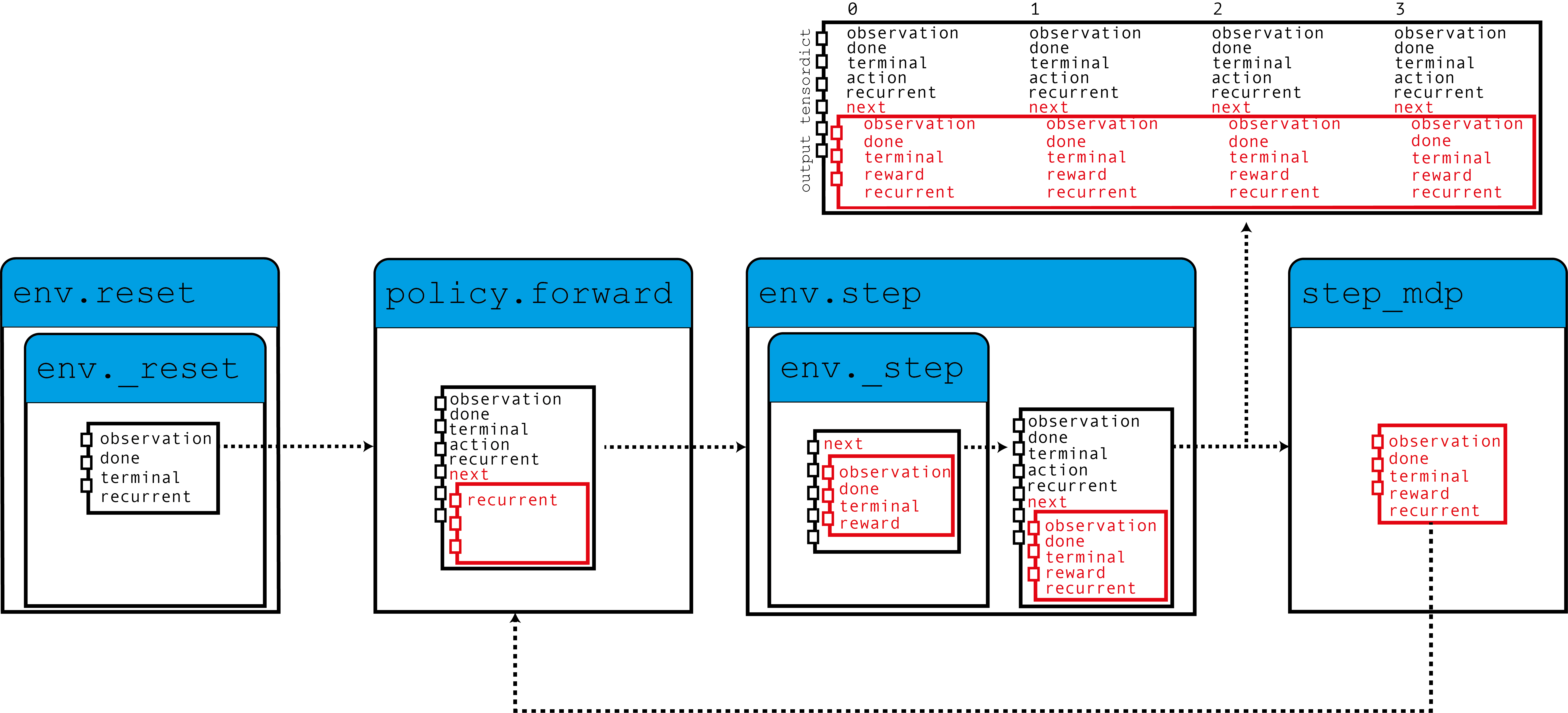
Data collection with a recurrent policy

如图所示,我们的环境使用归零的循环状态填充 TensorDict,策略读取这些状态以及观测结果以产生动作,以及将用于下一步的循环状态。当调用 step_mdp() 函数时,来自下一个状态的循环状态将被带到当前的 TensorDict 中。让我们看看这在实践中是如何实现的。

如果你在 Google Colab 中运行此代码,请确保安装以下依赖项

!pip3 install torchrl
!pip3 install gym[mujoco]
!pip3 install tqdm

设置

import torch
import tqdm
from tensordict.nn import TensorDictModule as Mod, TensorDictSequential as Seq
from torch import nn
from torchrl.collectors import SyncDataCollector
from torchrl.data import LazyMemmapStorage, TensorDictReplayBuffer
from torchrl.envs import (
    Compose,
    ExplorationType,
    GrayScale,
    InitTracker,
    ObservationNorm,
    Resize,
    RewardScaling,
    set_exploration_type,
    StepCounter,
    ToTensorImage,
    TransformedEnv,
)
from torchrl.envs.libs.gym import GymEnv
from torchrl.modules import ConvNet, EGreedyModule, LSTMModule, MLP, QValueModule
from torchrl.objectives import DQNLoss, SoftUpdate

is_fork = multiprocessing.get_start_method() == "fork"
device = (
    torch.device(0)
    if torch.cuda.is_available() and not is_fork
    else torch.device("cpu")
)

环境

和往常一样,第一步是构建我们的环境:它帮助我们定义问题并相应地构建策略网络。在本教程中,我们将运行 CartPole gym 环境的单个基于像素的实例,并进行一些自定义转换:转换为灰度、调整大小为 84x84、缩小奖励并标准化观测结果。

注意

StepCounter 变换是辅助的。由于 CartPole 任务的目标是使轨迹尽可能长,因此计算步数可以帮助我们跟踪策略的性能。

对于本教程的目的,以下两个变换很重要

  • InitTracker 将通过在 TensorDict 中添加 "is_init" 布尔掩码来标记对 reset() 的调用,该掩码将跟踪哪些步骤需要重置 RNN 隐藏状态。

  • TensorDictPrimer 变换稍微技术性一些。使用 RNN 策略不是必需的。但是,它指示环境(以及随后的收集器)预期会存在一些额外的键。添加后,调用 env.reset() 将使用归零张量填充 primer 中指示的条目。了解到策略期望这些张量,收集器将在收集期间传递它们。最终,我们将把隐藏状态存储在回放缓冲区中,这将帮助我们引导损失模块中 RNN 操作的计算(否则将以 0 初始化)。总结:不包括此变换不会对策略的训练产生巨大影响,但它会使循环键从收集的数据和回放缓冲区中消失,这反过来会导致训练略微欠佳。幸运的是,我们提出的 LSTMModule 配备了一个辅助方法来为我们构建该变换,因此我们可以等到构建它!

env = TransformedEnv(
    GymEnv("CartPole-v1", from_pixels=True, device=device),
    Compose(
        ToTensorImage(),
        GrayScale(),
        Resize(84, 84),
        StepCounter(),
        InitTracker(),
        RewardScaling(loc=0.0, scale=0.1),
        ObservationNorm(standard_normal=True, in_keys=["pixels"]),
    ),
)

和往常一样,我们需要手动初始化我们的归一化常数

env.transform[-1].init_stats(1000, reduce_dim=[0, 1, 2], cat_dim=0, keep_dims=[0])
td = env.reset()

策略

我们的策略将包含 3 个组件:一个 ConvNet 主干网络、一个 LSTMModule 内存层和一个浅层 MLP 块,该块将 LSTM 输出映射到动作值。

卷积神经网络

我们构建了一个卷积神经网络,两侧是 torch.nn.AdaptiveAvgPool2d,它将输出压缩为大小为 64 的向量。ConvNet 可以帮助我们实现这一点

feature = Mod(
    ConvNet(
        num_cells=[32, 32, 64],
        squeeze_output=True,
        aggregator_class=nn.AdaptiveAvgPool2d,
        aggregator_kwargs={"output_size": (1, 1)},
        device=device,
    ),
    in_keys=["pixels"],
    out_keys=["embed"],
)

我们在批量数据上执行第一个模块,以收集输出向量的大小

n_cells = feature(env.reset())["embed"].shape[-1]

LSTM 模块

TorchRL 提供了一个专门的 LSTMModule 类,用于在你的代码库中加入 LSTM。它是一个 TensorDictModuleBase 子类:因此,它有一组 in_keysout_keys,用于指示在模块执行期间应该期望读取和写入/更新哪些值。该类带有可自定义的预定义值,用于这些属性,以方便其构建。

注意

使用限制:此类几乎支持所有 LSTM 功能,例如 dropout 或多层 LSTM。但是,为了遵守 TorchRL 的约定,此 LSTM 必须将 batch_first 属性设置为 True,这不是 PyTorch 中的默认值。但是,我们的 LSTMModule 更改了此默认行为,因此我们可以使用本机调用。

此外,LSTM 不能将 bidirectional 属性设置为 True,因为这在在线设置中不可用。在这种情况下,默认值是正确的。

lstm = LSTMModule(
    input_size=n_cells,
    hidden_size=128,
    device=device,
    in_key="embed",
    out_key="embed",
)

让我们看一下 LSTM Module 类,特别是它的 in 和 out_keys

print("in_keys", lstm.in_keys)
print("out_keys", lstm.out_keys)
in_keys ['embed', 'recurrent_state_h', 'recurrent_state_c', 'is_init']
out_keys ['embed', ('next', 'recurrent_state_h'), ('next', 'recurrent_state_c')]

我们可以看到这些值包含我们指示为 in_key(和 out_key)的键以及循环键名称。 out_keys 前面有一个 “next” 前缀,指示它们需要写入 “next” TensorDict 中。我们使用此约定(可以通过传递 in_keys/out_keys 参数来覆盖)以确保调用 step_mdp() 会将循环状态移动到根 TensorDict,使其在后续调用期间可供 RNN 使用(参见引言中的图)。

如前所述,我们还需要向我们的环境添加一个可选的变换,以确保循环状态传递到缓冲区。make_tensordict_primer() 方法正是这样做的

env.append_transform(lstm.make_tensordict_primer())
TransformedEnv(
    env=GymEnv(env=CartPole-v1, batch_size=torch.Size([]), device=cuda:0),
    transform=Compose(
            ToTensorImage(keys=['pixels']),
            GrayScale(keys=['pixels']),
            Resize(w=84, h=84, interpolation=InterpolationMode.BILINEAR, keys=['pixels']),
            StepCounter(keys=[]),
            InitTracker(keys=[]),
            RewardScaling(loc=0.0000, scale=0.1000, keys=['reward']),
            ObservationNorm(keys=['pixels']),
            TensorDictPrimer(primers=Composite(
                recurrent_state_h: UnboundedContinuous(
                    shape=torch.Size([1, 128]),
                    space=ContinuousBox(
                        low=Tensor(shape=torch.Size([1, 128]), device=cuda:0, dtype=torch.float32, contiguous=True),
                        high=Tensor(shape=torch.Size([1, 128]), device=cuda:0, dtype=torch.float32, contiguous=True)),
                    device=cuda:0,
                    dtype=torch.float32,
                    domain=continuous),
                recurrent_state_c: UnboundedContinuous(
                    shape=torch.Size([1, 128]),
                    space=ContinuousBox(
                        low=Tensor(shape=torch.Size([1, 128]), device=cuda:0, dtype=torch.float32, contiguous=True),
                        high=Tensor(shape=torch.Size([1, 128]), device=cuda:0, dtype=torch.float32, contiguous=True)),
                    device=cuda:0,
                    dtype=torch.float32,
                    domain=continuous),
                device=cuda:0,
                shape=torch.Size([])), default_value={'recurrent_state_h': 0.0, 'recurrent_state_c': 0.0}, random=None)))

就是这样!我们可以打印环境以检查一切是否正常,现在我们已经添加了 primer

print(env)
TransformedEnv(
    env=GymEnv(env=CartPole-v1, batch_size=torch.Size([]), device=cuda:0),
    transform=Compose(
            ToTensorImage(keys=['pixels']),
            GrayScale(keys=['pixels']),
            Resize(w=84, h=84, interpolation=InterpolationMode.BILINEAR, keys=['pixels']),
            StepCounter(keys=[]),
            InitTracker(keys=[]),
            RewardScaling(loc=0.0000, scale=0.1000, keys=['reward']),
            ObservationNorm(keys=['pixels']),
            TensorDictPrimer(primers=Composite(
                recurrent_state_h: UnboundedContinuous(
                    shape=torch.Size([1, 128]),
                    space=ContinuousBox(
                        low=Tensor(shape=torch.Size([1, 128]), device=cuda:0, dtype=torch.float32, contiguous=True),
                        high=Tensor(shape=torch.Size([1, 128]), device=cuda:0, dtype=torch.float32, contiguous=True)),
                    device=cuda:0,
                    dtype=torch.float32,
                    domain=continuous),
                recurrent_state_c: UnboundedContinuous(
                    shape=torch.Size([1, 128]),
                    space=ContinuousBox(
                        low=Tensor(shape=torch.Size([1, 128]), device=cuda:0, dtype=torch.float32, contiguous=True),
                        high=Tensor(shape=torch.Size([1, 128]), device=cuda:0, dtype=torch.float32, contiguous=True)),
                    device=cuda:0,
                    dtype=torch.float32,
                    domain=continuous),
                device=cuda:0,
                shape=torch.Size([])), default_value={'recurrent_state_h': 0.0, 'recurrent_state_c': 0.0}, random=None)))

MLP

我们使用单层 MLP 来表示我们将用于策略的动作值。

mlp = MLP(
    out_features=2,
    num_cells=[
        64,
    ],
    device=device,
)

并用零填充偏差

mlp[-1].bias.data.fill_(0.0)
mlp = Mod(mlp, in_keys=["embed"], out_keys=["action_value"])

使用 Q 值选择动作

我们策略的最后一部分是 Q 值模块。 Q 值模块 QValueModule 将读取我们的 MLP 生成的 "action_values" 键,并从中收集具有最大值的动作。我们唯一需要做的是指定动作空间,这可以通过传递字符串或动作规范来完成。这使我们能够使用分类(有时称为“稀疏”)编码或其 one-hot 版本。

qval = QValueModule(spec=env.action_spec)

注意

TorchRL 还提供了一个包装器类 torchrl.modules.QValueActor,它将模块包装在一个 Sequential 中,以及一个 QValueModule,就像我们在此处显式执行的那样。这样做几乎没有什么优势,而且过程也不太透明,但最终结果将与我们在此处所做的类似。

我们现在可以将所有内容放在一个 TensorDictSequential

stoch_policy = Seq(feature, lstm, mlp, qval)

DQN 是一种确定性算法,探索是至关重要的一部分。我们将使用 \(\epsilon\)-greedy 策略,epsilon 值为 0.2,并逐步衰减到 0。这种衰减是通过调用 step() 实现的(参见下面的训练循环)。

exploration_module = EGreedyModule(
    annealing_num_steps=1_000_000, spec=env.action_spec, eps_init=0.2
)
stoch_policy = Seq(
    stoch_policy,
    exploration_module,
)

使用模型进行损失计算

我们构建的模型非常适合在顺序设置中使用。但是,类 torch.nn.LSTM 可以使用 cuDNN 优化的后端在 GPU 设备上更快地运行 RNN 序列。我们不想错过这样的机会来加速我们的训练循环!要使用它,我们只需要告诉 LSTM 模块在损失使用时以 “recurrent-mode” 运行。由于我们通常希望拥有 LSTM 模块的两个副本,因此我们通过调用 set_recurrent_mode() 方法来执行此操作,该方法将返回 LSTM 的新实例(具有共享权重),该实例将假定输入数据本质上是顺序的。

policy = Seq(feature, lstm.set_recurrent_mode(True), mlp, qval)

因为我们仍然有一些未初始化的参数,所以我们应该在创建优化器等之前初始化它们。

policy(env.reset())
TensorDict(
    fields={
        action: Tensor(shape=torch.Size([2]), device=cuda:0, dtype=torch.int64, is_shared=True),
        action_value: Tensor(shape=torch.Size([2]), device=cuda:0, dtype=torch.float32, is_shared=True),
        chosen_action_value: Tensor(shape=torch.Size([1]), device=cuda:0, dtype=torch.float32, is_shared=True),
        done: Tensor(shape=torch.Size([1]), device=cuda:0, dtype=torch.bool, is_shared=True),
        embed: Tensor(shape=torch.Size([128]), device=cuda:0, dtype=torch.float32, is_shared=True),
        is_init: Tensor(shape=torch.Size([1]), device=cuda:0, dtype=torch.bool, is_shared=True),
        next: TensorDict(
            fields={
                recurrent_state_c: Tensor(shape=torch.Size([1, 128]), device=cuda:0, dtype=torch.float32, is_shared=True),
                recurrent_state_h: Tensor(shape=torch.Size([1, 128]), device=cuda:0, dtype=torch.float32, is_shared=True)},
            batch_size=torch.Size([]),
            device=cuda:0,
            is_shared=True),
        pixels: Tensor(shape=torch.Size([1, 84, 84]), device=cuda:0, dtype=torch.float32, is_shared=True),
        recurrent_state_c: Tensor(shape=torch.Size([1, 128]), device=cuda:0, dtype=torch.float32, is_shared=True),
        recurrent_state_h: Tensor(shape=torch.Size([1, 128]), device=cuda:0, dtype=torch.float32, is_shared=True),
        step_count: Tensor(shape=torch.Size([1]), device=cuda:0, dtype=torch.int64, is_shared=True),
        terminated: Tensor(shape=torch.Size([1]), device=cuda:0, dtype=torch.bool, is_shared=True),
        truncated: Tensor(shape=torch.Size([1]), device=cuda:0, dtype=torch.bool, is_shared=True)},
    batch_size=torch.Size([]),
    device=cuda:0,
    is_shared=True)

DQN 损失

我们的 DQN 损失要求我们传递策略,以及再次传递动作空间。虽然这看起来可能是多余的,但这很重要,因为我们希望确保 DQNLossQValueModule 类是兼容的,但彼此之间并非强依赖。

要使用 Double-DQN,我们要求提供一个 delay_value 参数,该参数将创建网络参数的不可微分副本以用作目标网络。

loss_fn = DQNLoss(policy, action_space=env.action_spec, delay_value=True)

由于我们正在使用双重 DQN,因此我们需要更新目标参数。我们将使用 SoftUpdate 实例来执行这项工作。

updater = SoftUpdate(loss_fn, eps=0.95)

optim = torch.optim.Adam(policy.parameters(), lr=3e-4)

收集器和回放缓冲区

我们构建了最简单的数据收集器。我们将尝试使用一百万帧来训练我们的算法,每次扩展缓冲区 50 帧。缓冲区将设计为存储 20,000 个轨迹,每个轨迹 50 步。在每个优化步骤(每次数据收集 16 次)中,我们将从缓冲区中收集 4 个项目,总共 200 个转换。我们将使用 LazyMemmapStorage 存储来将数据保存在磁盘上。

注意

为了提高效率,我们在这里只运行几千次迭代。在实际设置中,总帧数应设置为 1M。

collector = SyncDataCollector(env, stoch_policy, frames_per_batch=50, total_frames=200, device=device)
rb = TensorDictReplayBuffer(
    storage=LazyMemmapStorage(20_000), batch_size=4, prefetch=10
)

训练循环

为了跟踪进度,我们将每 50 次数据收集在环境中运行一次策略,并在训练后绘制结果。

utd = 16
pbar = tqdm.tqdm(total=1_000_000)
longest = 0

traj_lens = []
for i, data in enumerate(collector):
    if i == 0:
        print(
            "Let us print the first batch of data.\nPay attention to the key names "
            "which will reflect what can be found in this data structure, in particular: "
            "the output of the QValueModule (action_values, action and chosen_action_value),"
            "the 'is_init' key that will tell us if a step is initial or not, and the "
            "recurrent_state keys.\n",
            data,
        )
    pbar.update(data.numel())
    # it is important to pass data that is not flattened
    rb.extend(data.unsqueeze(0).to_tensordict().cpu())
    for _ in range(utd):
        s = rb.sample().to(device, non_blocking=True)
        loss_vals = loss_fn(s)
        loss_vals["loss"].backward()
        optim.step()
        optim.zero_grad()
    longest = max(longest, data["step_count"].max().item())
    pbar.set_description(
        f"steps: {longest}, loss_val: {loss_vals['loss'].item(): 4.4f}, action_spread: {data['action'].sum(0)}"
    )
    exploration_module.step(data.numel())
    updater.step()

    with set_exploration_type(ExplorationType.DETERMINISTIC), torch.no_grad():
        rollout = env.rollout(10000, stoch_policy)
        traj_lens.append(rollout.get(("next", "step_count")).max().item())
  0%|          | 0/1000000 [00:00<?, ?it/s]Let us print the first batch of data.
Pay attention to the key names which will reflect what can be found in this data structure, in particular: the output of the QValueModule (action_values, action and chosen_action_value),the 'is_init' key that will tell us if a step is initial or not, and the recurrent_state keys.
 TensorDict(
    fields={
        action: Tensor(shape=torch.Size([50, 2]), device=cuda:0, dtype=torch.int64, is_shared=True),
        action_value: Tensor(shape=torch.Size([50, 2]), device=cuda:0, dtype=torch.float32, is_shared=True),
        chosen_action_value: Tensor(shape=torch.Size([50, 1]), device=cuda:0, dtype=torch.float32, is_shared=True),
        collector: TensorDict(
            fields={
                traj_ids: Tensor(shape=torch.Size([50]), device=cuda:0, dtype=torch.int64, is_shared=True)},
            batch_size=torch.Size([50]),
            device=cuda:0,
            is_shared=True),
        done: Tensor(shape=torch.Size([50, 1]), device=cuda:0, dtype=torch.bool, is_shared=True),
        embed: Tensor(shape=torch.Size([50, 128]), device=cuda:0, dtype=torch.float32, is_shared=True),
        is_init: Tensor(shape=torch.Size([50, 1]), device=cuda:0, dtype=torch.bool, is_shared=True),
        next: TensorDict(
            fields={
                done: Tensor(shape=torch.Size([50, 1]), device=cuda:0, dtype=torch.bool, is_shared=True),
                is_init: Tensor(shape=torch.Size([50, 1]), device=cuda:0, dtype=torch.bool, is_shared=True),
                pixels: Tensor(shape=torch.Size([50, 1, 84, 84]), device=cuda:0, dtype=torch.float32, is_shared=True),
                recurrent_state_c: Tensor(shape=torch.Size([50, 1, 128]), device=cuda:0, dtype=torch.float32, is_shared=True),
                recurrent_state_h: Tensor(shape=torch.Size([50, 1, 128]), device=cuda:0, dtype=torch.float32, is_shared=True),
                reward: Tensor(shape=torch.Size([50, 1]), device=cuda:0, dtype=torch.float32, is_shared=True),
                step_count: Tensor(shape=torch.Size([50, 1]), device=cuda:0, dtype=torch.int64, is_shared=True),
                terminated: Tensor(shape=torch.Size([50, 1]), device=cuda:0, dtype=torch.bool, is_shared=True),
                truncated: Tensor(shape=torch.Size([50, 1]), device=cuda:0, dtype=torch.bool, is_shared=True)},
            batch_size=torch.Size([50]),
            device=cuda:0,
            is_shared=True),
        pixels: Tensor(shape=torch.Size([50, 1, 84, 84]), device=cuda:0, dtype=torch.float32, is_shared=True),
        recurrent_state_c: Tensor(shape=torch.Size([50, 1, 128]), device=cuda:0, dtype=torch.float32, is_shared=True),
        recurrent_state_h: Tensor(shape=torch.Size([50, 1, 128]), device=cuda:0, dtype=torch.float32, is_shared=True),
        step_count: Tensor(shape=torch.Size([50, 1]), device=cuda:0, dtype=torch.int64, is_shared=True),
        terminated: Tensor(shape=torch.Size([50, 1]), device=cuda:0, dtype=torch.bool, is_shared=True),
        truncated: Tensor(shape=torch.Size([50, 1]), device=cuda:0, dtype=torch.bool, is_shared=True)},
    batch_size=torch.Size([50]),
    device=cuda:0,
    is_shared=True)

  0%|          | 50/1000000 [00:00<1:27:22, 190.76it/s]
steps: 12, loss_val:  0.0004, action_spread: tensor([47,  3], device='cuda:0'):   0%|          | 50/1000000 [00:01<1:27:22, 190.76it/s]
steps: 12, loss_val:  0.0004, action_spread: tensor([47,  3], device='cuda:0'):   0%|          | 100/1000000 [00:01<5:16:29, 52.66it/s]
steps: 12, loss_val:  0.0003, action_spread: tensor([46,  4], device='cuda:0'):   0%|          | 100/1000000 [00:02<5:16:29, 52.66it/s]
steps: 12, loss_val:  0.0003, action_spread: tensor([46,  4], device='cuda:0'):   0%|          | 150/1000000 [00:02<5:43:36, 48.50it/s]
steps: 12, loss_val:  0.0002, action_spread: tensor([44,  6], device='cuda:0'):   0%|          | 150/1000000 [00:03<5:43:36, 48.50it/s]
steps: 12, loss_val:  0.0002, action_spread: tensor([44,  6], device='cuda:0'):   0%|          | 200/1000000 [00:04<6:04:34, 45.71it/s]
steps: 19, loss_val:  0.0002, action_spread: tensor([ 6, 44], device='cuda:0'):   0%|          | 200/1000000 [00:04<6:04:34, 45.71it/s]

让我们绘制结果

if traj_lens:
    from matplotlib import pyplot as plt

    plt.plot(traj_lens)
    plt.xlabel("Test collection")
    plt.title("Test trajectory lengths")
Test trajectory lengths

结论

我们已经了解了如何在 TorchRL 的策略中加入 RNN。现在你应该能够

  • 创建一个充当 TensorDictModule 的 LSTM 模块

  • 通过 InitTracker 变换向 LSTM 模块指示需要重置

  • 将此模块合并到策略和损失模块中

  • 确保收集器知道循环状态条目,以便可以将它们与其余数据一起存储在回放缓冲区中

进一步阅读

  • TorchRL 文档可以在 此处 找到。

脚本的总运行时间: ( 0 分钟 9.009 秒)

由 Sphinx-Gallery 生成的图库


评价本教程

© 版权所有 2024,PyTorch。

使用 Sphinx 构建,主题由 theme 提供,托管于 Read the Docs

文档

访问 PyTorch 的全面开发者文档

查看文档

教程

获取面向初学者和高级开发者的深入教程

查看教程

资源

查找开发资源并获得问题解答

查看资源