注意

点击此处下载完整示例代码

神经网络¶

创建时间：2017年3月24日 | 最后更新：2024年5月6日 | 最后验证：2024年11月5日

神经网络可以使用 torch.nn 包构建。

既然您已经对 autograd 有所了解，nn 依赖于 autograd 来定义模型并对其进行微分。一个 nn.Module 包含层，以及一个 forward(input) 方法，该方法返回 output。

例如，看看这个对数字图像进行分类的网络

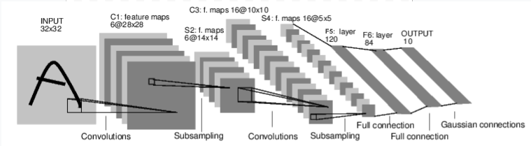
卷积网络¶

它是一个简单的全连接前馈网络。它接收输入，将其依次通过多个层，最后给出输出。

神经网络的典型训练过程如下

定义具有一些可学习参数（或权重）的神经网络
迭代输入数据集
通过网络处理输入
计算损失（输出与正确结果相差多远）
将梯度反向传播到网络的参数中
更新网络的权重，通常使用简单的更新规则：weight = weight - learning_rate * gradient

定义网络¶

让我们定义这个网络

import torch
import torch.nn as nn
import torch.nn.functional as F


class Net(nn.Module):

    def __init__(self):
        super(Net, self).__init__()
        # 1 input image channel, 6 output channels, 5x5 square convolution
        # kernel
        self.conv1 = nn.Conv2d(1, 6, 5)
        self.conv2 = nn.Conv2d(6, 16, 5)
        # an affine operation: y = Wx + b
        self.fc1 = nn.Linear(16 * 5 * 5, 120)  # 5*5 from image dimension
        self.fc2 = nn.Linear(120, 84)
        self.fc3 = nn.Linear(84, 10)

    def forward(self, input):
        # Convolution layer C1: 1 input image channel, 6 output channels,
        # 5x5 square convolution, it uses RELU activation function, and
        # outputs a Tensor with size (N, 6, 28, 28), where N is the size of the batch
        c1 = F.relu(self.conv1(input))
        # Subsampling layer S2: 2x2 grid, purely functional,
        # this layer does not have any parameter, and outputs a (N, 6, 14, 14) Tensor
        s2 = F.max_pool2d(c1, (2, 2))
        # Convolution layer C3: 6 input channels, 16 output channels,
        # 5x5 square convolution, it uses RELU activation function, and
        # outputs a (N, 16, 10, 10) Tensor
        c3 = F.relu(self.conv2(s2))
        # Subsampling layer S4: 2x2 grid, purely functional,
        # this layer does not have any parameter, and outputs a (N, 16, 5, 5) Tensor
        s4 = F.max_pool2d(c3, 2)
        # Flatten operation: purely functional, outputs a (N, 400) Tensor
        s4 = torch.flatten(s4, 1)
        # Fully connected layer F5: (N, 400) Tensor input,
        # and outputs a (N, 120) Tensor, it uses RELU activation function
        f5 = F.relu(self.fc1(s4))
        # Fully connected layer F6: (N, 120) Tensor input,
        # and outputs a (N, 84) Tensor, it uses RELU activation function
        f6 = F.relu(self.fc2(f5))
        # Gaussian layer OUTPUT: (N, 84) Tensor input, and
        # outputs a (N, 10) Tensor
        output = self.fc3(f6)
        return output


net = Net()
print(net)

Net(
  (conv1): Conv2d(1, 6, kernel_size=(5, 5), stride=(1, 1))
  (conv2): Conv2d(6, 16, kernel_size=(5, 5), stride=(1, 1))
  (fc1): Linear(in_features=400, out_features=120, bias=True)
  (fc2): Linear(in_features=120, out_features=84, bias=True)
  (fc3): Linear(in_features=84, out_features=10, bias=True)
)

您只需定义 forward 函数，而 backward 函数（计算梯度的地方）会使用 autograd 自动为您定义。您可以在 forward 函数中使用任何 Tensor 操作。

模型的可学习参数由 net.parameters() 返回

params = list(net.parameters())
print(len(params))
print(params[0].size())  # conv1's .weight

10
torch.Size([6, 1, 5, 5])

让我们尝试一个随机的 32x32 输入。注意：该网络 (LeNet) 的预期输入大小是 32x32。要在 MNIST 数据集上使用此网络，请将数据集中的图像大小调整为 32x32。

input = torch.randn(1, 1, 32, 32)
out = net(input)
print(out)

tensor([[ 0.1453, -0.0590, -0.0065,  0.0905,  0.0146, -0.0805, -0.1211, -0.0394,
         -0.0181, -0.0136]], grad_fn=<AddmmBackward0>)

将所有参数的梯度缓冲区清零，并使用随机梯度进行反向传播

net.zero_grad()
out.backward(torch.randn(1, 10))

注意

torch.nn 只支持 mini-batch。整个 torch.nn 包只支持输入是样本的 mini-batch，而不是单个样本。

例如，nn.Conv2d 将接收一个形状为 nSamples x nChannels x Height x Width 的 4D Tensor。

如果您有一个单个样本，只需使用 input.unsqueeze(0) 来添加一个伪造的 batch 维度。

在继续之前，让我们回顾一下目前为止您所见过的所有类。

回顾

torch.Tensor - 一个支持 backward() 等 autograd 操作的多维数组。也持有关于该张量的梯度。
nn.Module - 神经网络模块。一种方便封装参数的方式，并提供将参数移动到 GPU、导出、加载等辅助功能。
nn.Parameter - 一种 Tensor，在被赋值为 Module 的属性时会自动注册为参数。
autograd.Function - 实现autograd 操作的前向和后向定义。每个 Tensor 操作都会创建至少一个 Function 节点，该节点连接到创建该 Tensor 的函数，并编码其历史。

至此，我们已经涵盖了

定义神经网络
处理输入并调用 backward

剩余部分

计算损失
更新网络权重

损失函数¶

损失函数接收 (输出, 目标) 对作为输入，并计算一个值来估计输出与目标之间的距离。

nn 包下有几种不同的损失函数。一个简单的损失函数是：nn.MSELoss，它计算输出和目标之间的均方误差。

例如

output = net(input)
target = torch.randn(10)  # a dummy target, for example
target = target.view(1, -1)  # make it the same shape as output
criterion = nn.MSELoss()

loss = criterion(output, target)
print(loss)

tensor(1.3619, grad_fn=<MseLossBackward0>)

现在，如果您使用 loss 的 .grad_fn 属性沿着反向方向跟踪，您会看到一个计算图，看起来像这样

input -> conv2d -> relu -> maxpool2d -> conv2d -> relu -> maxpool2d
      -> flatten -> linear -> relu -> linear -> relu -> linear
      -> MSELoss
      -> loss

因此，当我们调用 loss.backward() 时，整个图将相对于神经网络参数进行微分，并且图中所有 requires_grad=True 的 Tensor 的 .grad Tensor 将累积梯度。

作为说明，让我们向后跟踪几个步骤

print(loss.grad_fn)  # MSELoss
print(loss.grad_fn.next_functions[0][0])  # Linear
print(loss.grad_fn.next_functions[0][0].next_functions[0][0])  # ReLU

<MseLossBackward0 object at 0x7fbc2e2a7eb0>
<AddmmBackward0 object at 0x7fbc2e2a78e0>
<AccumulateGrad object at 0x7fbc2e2a7b80>

反向传播¶

要反向传播误差，我们只需调用 loss.backward()。但是，您需要清除现有的梯度，否则梯度会累积到现有梯度中。

现在我们将调用 loss.backward()，并查看 conv1 的 bias 梯度在反向传播之前和之后的变化。

net.zero_grad()     # zeroes the gradient buffers of all parameters

print('conv1.bias.grad before backward')
print(net.conv1.bias.grad)

loss.backward()

print('conv1.bias.grad after backward')
print(net.conv1.bias.grad)

conv1.bias.grad before backward
None
conv1.bias.grad after backward
tensor([ 0.0081, -0.0080, -0.0039,  0.0150,  0.0003, -0.0105])

现在，我们已经了解了如何使用损失函数。

稍后阅读

神经网络包包含各种模块和损失函数，它们构成了深度神经网络的构建块。包含文档的完整列表在此处。

剩下的唯一需要学习的是

更新网络权重

更新权重¶

实践中最简单的更新规则是随机梯度下降 (SGD)

weight = weight - learning_rate * gradient

我们可以使用简单的 Python 代码来实现这一点

learning_rate = 0.01
for f in net.parameters():
    f.data.sub_(f.grad.data * learning_rate)

然而，在使用神经网络时，您会想要使用各种不同的更新规则，例如 SGD、Nesterov-SGD、Adam、RMSProp 等。为了实现这一点，我们构建了一个小型包：torch.optim，它实现了所有这些方法。使用它非常简单

import torch.optim as optim

# create your optimizer
optimizer = optim.SGD(net.parameters(), lr=0.01)

# in your training loop:
optimizer.zero_grad()   # zero the gradient buffers
output = net(input)
loss = criterion(output, target)
loss.backward()
optimizer.step()    # Does the update

注意

请注意，必须使用 optimizer.zero_grad() 手动将梯度缓冲区设置为零。这是因为正如反向传播部分所解释的，梯度是累积的。

脚本总运行时间： ( 0 分钟 0.137 秒)

由 Sphinx-Gallery 生成的画廊