注意

点击此处下载完整示例代码

Torchaudio-Squim: TorchAudio 中的非侵入式语音评估¶

作者：Anurag Kumar, Zhaoheng Ni

1. 概述¶

本教程展示了如何使用 Torchaudio-Squim 估计客观和主观指标，用于评估语音质量和可懂度。

TorchAudio-Squim 在 Torchaudio 中提供了语音评估功能。它提供接口和预训练模型，用于估计各种语音质量和可懂度指标。目前，Torchaudio-Squim [1] 支持对 3 个广泛使用的客观指标进行无参考估计：

Wideband Perceptual Estimation of Speech Quality (PESQ) [2]（宽带感知语音质量评估）
Short-Time Objective Intelligibility (STOI) [3]（短时客观可懂度）
Scale-Invariant Signal-to-Distortion Ratio (SI-SDR) [4]（尺度不变信号失真比）

它还支持使用非匹配参考 (Non-Matching References) [1, 5] 估计给定音频波形的主观平均主观意见得分 (MOS)。

参考

[1] Kumar, Anurag, et al. “TorchAudio-Squim: Reference-less Speech Quality and Intelligibility measures in TorchAudio.” ICASSP 2023-2023 IEEE International Conference on Acoustics, Speech and Signal Processing (ICASSP). IEEE, 2023.

[2] I. Rec, “P.862.2: Wideband extension to recommendation P.862 for the assessment of wideband telephone networks and speech codecs,” International Telecommunication Union, CH–Geneva, 2005.

[3] Taal, C. H., Hendriks, R. C., Heusdens, R., & Jensen, J. (2010, March). A short-time objective intelligibility measure for time-frequency weighted noisy speech. In 2010 IEEE international conference on acoustics, speech and signal processing (pp. 4214-4217). IEEE.

[4] Le Roux, Jonathan, et al. “SDR–half-baked or well done?.” ICASSP 2019-2019 IEEE International Conference on Acoustics, Speech and Signal Processing (ICASSP). IEEE, 2019.

[5] Manocha, Pranay, and Anurag Kumar. “Speech quality assessment through MOS using non-matching references.” Interspeech, 2022.

import torch
import torchaudio

print(torch.__version__)
print(torchaudio.__version__)

2.7.0
2.7.0

2. 准备工作¶

首先导入模块并定义辅助函数。

我们将需要 torch、torchaudio 来使用 Torchaudio-squim，Matplotlib 用于绘图，pystoi、pesq 用于计算参考指标。

try:
    from pesq import pesq
    from pystoi import stoi
    from torchaudio.pipelines import SQUIM_OBJECTIVE, SQUIM_SUBJECTIVE
except ImportError:
    try:
        import google.colab  # noqa: F401

        print(
            """
            To enable running this notebook in Google Colab, install nightly
            torch and torchaudio builds by adding the following code block to the top
            of the notebook before running it:
            !pip3 uninstall -y torch torchvision torchaudio
            !pip3 install --pre torch torchvision torchaudio --extra-index-url https://download.pytorch.org/whl/nightly/cpu
            !pip3 install pesq
            !pip3 install pystoi
            """
        )
    except Exception:
        pass
    raise


import matplotlib.pyplot as plt

import torchaudio.functional as F
from IPython.display import Audio
from torchaudio.utils import download_asset


def si_snr(estimate, reference, epsilon=1e-8):
    estimate = estimate - estimate.mean()
    reference = reference - reference.mean()
    reference_pow = reference.pow(2).mean(axis=1, keepdim=True)
    mix_pow = (estimate * reference).mean(axis=1, keepdim=True)
    scale = mix_pow / (reference_pow + epsilon)

    reference = scale * reference
    error = estimate - reference

    reference_pow = reference.pow(2)
    error_pow = error.pow(2)

    reference_pow = reference_pow.mean(axis=1)
    error_pow = error_pow.mean(axis=1)

    si_snr = 10 * torch.log10(reference_pow) - 10 * torch.log10(error_pow)
    return si_snr.item()


def plot(waveform, title, sample_rate=16000):
    wav_numpy = waveform.numpy()

    sample_size = waveform.shape[1]
    time_axis = torch.arange(0, sample_size) / sample_rate

    figure, axes = plt.subplots(2, 1)
    axes[0].plot(time_axis, wav_numpy[0], linewidth=1)
    axes[0].grid(True)
    axes[1].specgram(wav_numpy[0], Fs=sample_rate)
    figure.suptitle(title)

3. 加载语音和噪声样本¶

SAMPLE_SPEECH = download_asset("tutorial-assets/Lab41-SRI-VOiCES-src-sp0307-ch127535-sg0042.wav")
SAMPLE_NOISE = download_asset("tutorial-assets/Lab41-SRI-VOiCES-rm1-babb-mc01-stu-clo.wav")

  0%|          | 0.00/156k [00:00<?, ?B/s]
100%|##########| 156k/156k [00:00<00:00, 65.3MB/s]

WAVEFORM_SPEECH, SAMPLE_RATE_SPEECH = torchaudio.load(SAMPLE_SPEECH)
WAVEFORM_NOISE, SAMPLE_RATE_NOISE = torchaudio.load(SAMPLE_NOISE)
WAVEFORM_NOISE = WAVEFORM_NOISE[0:1, :]

目前，Torchaudio-Squim 模型仅支持 16000 Hz 采样率。如有必要，对波形进行重采样。

if SAMPLE_RATE_SPEECH != 16000:
    WAVEFORM_SPEECH = F.resample(WAVEFORM_SPEECH, SAMPLE_RATE_SPEECH, 16000)

if SAMPLE_RATE_NOISE != 16000:
    WAVEFORM_NOISE = F.resample(WAVEFORM_NOISE, SAMPLE_RATE_NOISE, 16000)

修剪波形，使其具有相同数量的帧。

if WAVEFORM_SPEECH.shape[1] < WAVEFORM_NOISE.shape[1]:
    WAVEFORM_NOISE = WAVEFORM_NOISE[:, : WAVEFORM_SPEECH.shape[1]]
else:
    WAVEFORM_SPEECH = WAVEFORM_SPEECH[:, : WAVEFORM_NOISE.shape[1]]

播放语音样本

Audio(WAVEFORM_SPEECH.numpy()[0], rate=16000)

播放噪声样本

Audio(WAVEFORM_NOISE.numpy()[0], rate=16000)

4. 创建失真（带噪）语音样本¶

snr_dbs = torch.tensor([20, -5])
WAVEFORM_DISTORTED = F.add_noise(WAVEFORM_SPEECH, WAVEFORM_NOISE, snr_dbs)

播放信噪比为 20dB 的失真语音

Audio(WAVEFORM_DISTORTED.numpy()[0], rate=16000)

播放信噪比为 -5dB 的失真语音

Audio(WAVEFORM_DISTORTED.numpy()[1], rate=16000)

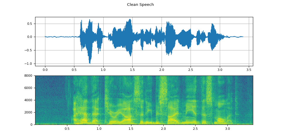
5. 可视化波形¶

可视化语音样本

plot(WAVEFORM_SPEECH, "Clean Speech")

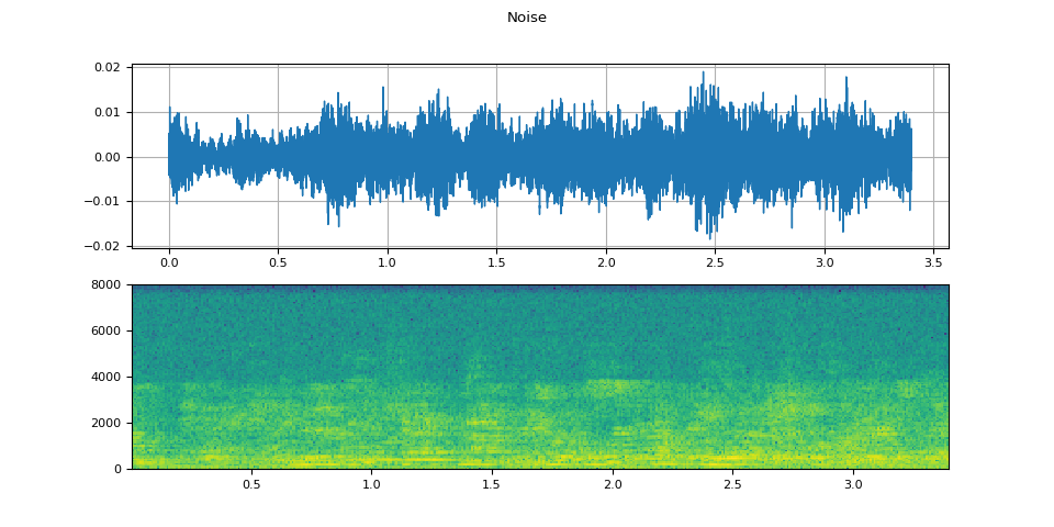
可视化噪声样本

plot(WAVEFORM_NOISE, "Noise")

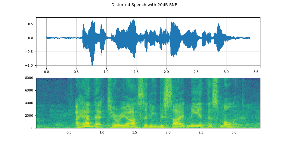
可视化信噪比为 20dB 的失真语音

plot(WAVEFORM_DISTORTED[0:1], f"Distorted Speech with {snr_dbs[0]}dB SNR")

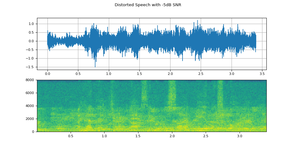
可视化信噪比为 -5dB 的失真语音

plot(WAVEFORM_DISTORTED[1:2], f"Distorted Speech with {snr_dbs[1]}dB SNR")

6. 预测客观指标¶

获取预训练的 SquimObjective 模型。

objective_model = SQUIM_OBJECTIVE.get_model()

  0%|          | 0.00/28.2M [00:00<?, ?B/s]
 52%|#####2    | 14.8M/28.2M [00:00<00:00, 27.7MB/s]
 62%|######2   | 17.5M/28.2M [00:00<00:00, 22.5MB/s]
 96%|#########5| 27.0M/28.2M [00:00<00:00, 31.0MB/s]
100%|##########| 28.2M/28.2M [00:00<00:00, 29.9MB/s]

将模型输出与信噪比为 20dB 的失真语音的真实值进行比较

stoi_hyp, pesq_hyp, si_sdr_hyp = objective_model(WAVEFORM_DISTORTED[0:1, :])
print(f"Estimated metrics for distorted speech at {snr_dbs[0]}dB are\n")
print(f"STOI: {stoi_hyp[0]}")
print(f"PESQ: {pesq_hyp[0]}")
print(f"SI-SDR: {si_sdr_hyp[0]}\n")

pesq_ref = pesq(16000, WAVEFORM_SPEECH[0].numpy(), WAVEFORM_DISTORTED[0].numpy(), mode="wb")
stoi_ref = stoi(WAVEFORM_SPEECH[0].numpy(), WAVEFORM_DISTORTED[0].numpy(), 16000, extended=False)
si_sdr_ref = si_snr(WAVEFORM_DISTORTED[0:1], WAVEFORM_SPEECH)
print(f"Reference metrics for distorted speech at {snr_dbs[0]}dB are\n")
print(f"STOI: {stoi_ref}")
print(f"PESQ: {pesq_ref}")
print(f"SI-SDR: {si_sdr_ref}")

Estimated metrics for distorted speech at 20dB are

STOI: 0.9610356092453003
PESQ: 2.7801527976989746
SI-SDR: 20.692630767822266

Reference metrics for distorted speech at 20dB are

STOI: 0.9670831113894452
PESQ: 2.7961528301239014
SI-SDR: 19.998966217041016

将模型输出与信噪比为 -5dB 的失真语音的真实值进行比较

stoi_hyp, pesq_hyp, si_sdr_hyp = objective_model(WAVEFORM_DISTORTED[1:2, :])
print(f"Estimated metrics for distorted speech at {snr_dbs[1]}dB are\n")
print(f"STOI: {stoi_hyp[0]}")
print(f"PESQ: {pesq_hyp[0]}")
print(f"SI-SDR: {si_sdr_hyp[0]}\n")

pesq_ref = pesq(16000, WAVEFORM_SPEECH[0].numpy(), WAVEFORM_DISTORTED[1].numpy(), mode="wb")
stoi_ref = stoi(WAVEFORM_SPEECH[0].numpy(), WAVEFORM_DISTORTED[1].numpy(), 16000, extended=False)
si_sdr_ref = si_snr(WAVEFORM_DISTORTED[1:2], WAVEFORM_SPEECH)
print(f"Reference metrics for distorted speech at {snr_dbs[1]}dB are\n")
print(f"STOI: {stoi_ref}")
print(f"PESQ: {pesq_ref}")
print(f"SI-SDR: {si_sdr_ref}")

Estimated metrics for distorted speech at -5dB are

STOI: 0.5743248462677002
PESQ: 1.1112866401672363
SI-SDR: -6.248741626739502

Reference metrics for distorted speech at -5dB are

STOI: 0.5848137931588825
PESQ: 1.0803768634796143
SI-SDR: -5.016279220581055

7. 预测平均主观意见得分（主观指标）¶

获取预训练的 SquimSubjective 模型。

subjective_model = SQUIM_SUBJECTIVE.get_model()

  0%|          | 0.00/360M [00:00<?, ?B/s]
  1%|          | 2.12M/360M [00:00<00:18, 19.8MB/s]
  2%|1         | 6.38M/360M [00:00<00:13, 27.3MB/s]
  2%|2         | 9.00M/360M [00:00<00:18, 19.6MB/s]
  4%|3         | 12.8M/360M [00:00<00:16, 22.0MB/s]
  5%|4         | 16.5M/360M [00:00<00:16, 22.2MB/s]
  9%|8         | 31.1M/360M [00:01<00:09, 35.6MB/s]
 10%|9         | 34.2M/360M [00:01<00:11, 29.1MB/s]
 13%|#3        | 47.6M/360M [00:01<00:06, 47.3MB/s]
 15%|#4        | 52.9M/360M [00:01<00:08, 38.3MB/s]
 18%|#8        | 65.6M/360M [00:01<00:06, 48.0MB/s]
 22%|##2       | 79.2M/360M [00:01<00:04, 65.3MB/s]
 24%|##4       | 87.0M/360M [00:02<00:05, 48.9MB/s]
 27%|##6       | 96.8M/360M [00:02<00:04, 55.9MB/s]
 29%|##8       | 104M/360M [00:02<00:05, 49.8MB/s]
 32%|###1      | 115M/360M [00:02<00:04, 55.5MB/s]
 35%|###5      | 126M/360M [00:02<00:03, 68.5MB/s]
 37%|###7      | 134M/360M [00:03<00:04, 50.8MB/s]
 41%|####      | 146M/360M [00:03<00:03, 60.5MB/s]
 42%|####2     | 153M/360M [00:03<00:04, 54.1MB/s]
 45%|####5     | 164M/360M [00:03<00:03, 55.3MB/s]
 48%|####8     | 174M/360M [00:03<00:02, 65.3MB/s]
 50%|#####     | 182M/360M [00:03<00:03, 54.2MB/s]
 54%|#####4    | 195M/360M [00:04<00:03, 55.5MB/s]
 56%|#####5    | 201M/360M [00:04<00:03, 49.3MB/s]
 59%|#####8    | 211M/360M [00:04<00:02, 55.0MB/s]
 60%|######    | 217M/360M [00:04<00:03, 48.8MB/s]
 63%|######3   | 228M/360M [00:04<00:02, 59.4MB/s]
 65%|######5   | 234M/360M [00:04<00:02, 56.1MB/s]
 68%|######7   | 244M/360M [00:05<00:02, 59.7MB/s]
 69%|######9   | 250M/360M [00:05<00:02, 55.5MB/s]
 72%|#######2  | 260M/360M [00:05<00:01, 65.3MB/s]
 74%|#######3  | 266M/360M [00:05<00:02, 45.0MB/s]
 77%|#######6  | 277M/360M [00:05<00:01, 43.7MB/s]
 78%|#######8  | 282M/360M [00:06<00:02, 32.2MB/s]
 79%|#######9  | 286M/360M [00:06<00:02, 30.9MB/s]
 82%|########1 | 294M/360M [00:06<00:01, 40.3MB/s]
 83%|########3 | 300M/360M [00:06<00:01, 40.8MB/s]
 86%|########6 | 311M/360M [00:06<00:01, 48.6MB/s]
 91%|######### | 328M/360M [00:07<00:00, 59.7MB/s]
 95%|#########5| 342M/360M [00:07<00:00, 67.7MB/s]
 97%|#########6| 349M/360M [00:07<00:00, 59.4MB/s]
100%|#########9| 359M/360M [00:07<00:00, 66.7MB/s]
100%|##########| 360M/360M [00:07<00:00, 50.2MB/s]

加载非匹配参考 (NMR)

NMR_SPEECH = download_asset("tutorial-assets/ctc-decoding/1688-142285-0007.wav")

WAVEFORM_NMR, SAMPLE_RATE_NMR = torchaudio.load(NMR_SPEECH)
if SAMPLE_RATE_NMR != 16000:
    WAVEFORM_NMR = F.resample(WAVEFORM_NMR, SAMPLE_RATE_NMR, 16000)

计算信噪比为 20dB 的失真语音的 MOS 指标

mos = subjective_model(WAVEFORM_DISTORTED[0:1, :], WAVEFORM_NMR)
print(f"Estimated MOS for distorted speech at {snr_dbs[0]}dB is MOS: {mos[0]}")

Estimated MOS for distorted speech at 20dB is MOS: 4.309267997741699

计算信噪比为 -5dB 的失真语音的 MOS 指标

mos = subjective_model(WAVEFORM_DISTORTED[1:2, :], WAVEFORM_NMR)
print(f"Estimated MOS for distorted speech at {snr_dbs[1]}dB is MOS: {mos[0]}")

Estimated MOS for distorted speech at -5dB is MOS: 3.291804075241089

8. 与真实值和基线进行比较¶

可视化 SquimObjective 和 SquimSubjective 模型估计的指标，可以帮助用户更好地理解这些模型在实际场景中的应用方式。下图显示了三种不同系统的散点图：MOSA-Net [1]、AMSA [2] 和 SquimObjective 模型，其中 y 轴表示估计的 STOI、PESQ 和 Si-SDR 分数，x 轴表示对应的真实值。

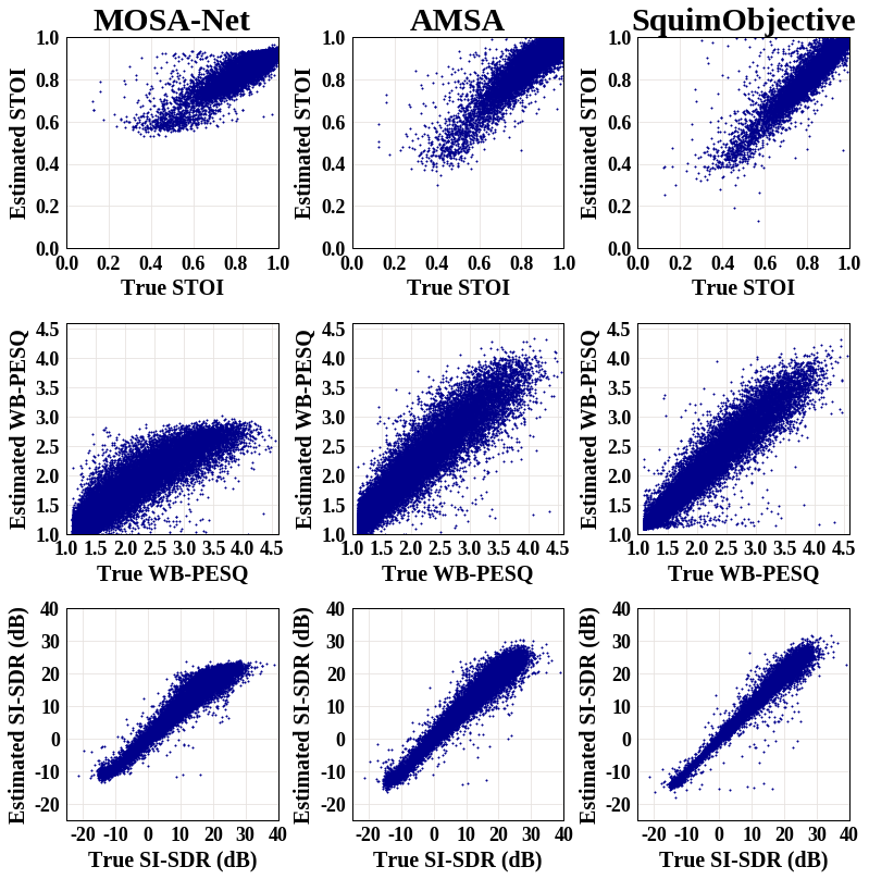
https://download.pytorch.org/torchaudio/tutorial-assets/objective_plot.png

[1] Zezario, Ryandhimas E., Szu-Wei Fu, Fei Chen, Chiou-Shann Fuh, Hsin-Min Wang, and Yu Tsao. “Deep learning-based non-intrusive multi-objective speech assessment model with cross-domain features.” IEEE/ACM Transactions on Audio, Speech, and Language Processing 31 (2022): 54-70.

[2] Dong, Xuan, and Donald S. Williamson. “An attention enhanced multi-task model for objective speech assessment in real-world environments.” In ICASSP 2020-2020 IEEE International Conference on Acoustics, Speech and Signal Processing (ICASSP), pp. 911-915. IEEE, 2020.

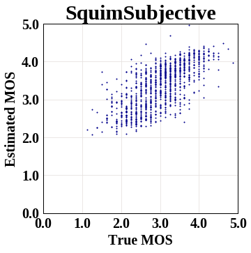
下图显示了 SquimSubjective 模型的散点图，其中 y 轴表示估计的 MOS 指标分数，x 轴表示对应的真实值。

https://download.pytorch.org/torchaudio/tutorial-assets/subjective_plot.png

脚本总运行时间： (0 分 14.618 秒)

由 Sphinx-Gallery 生成的图集