可视化工具

注意

在 Colab 上尝试 或 跳转至末尾 下载完整示例代码。

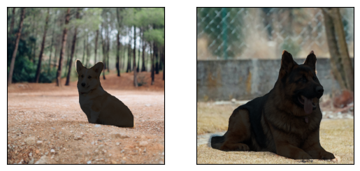
此示例演示了 torchvision 提供的一些用于可视化图像、边界框、分割掩码和关键点的工具函数。

import torch
import numpy as np
import matplotlib.pyplot as plt

import torchvision.transforms.functional as F


plt.rcParams["savefig.bbox"] = 'tight'


def show(imgs):
    if not isinstance(imgs, list):
        imgs = [imgs]
    fig, axs = plt.subplots(ncols=len(imgs), squeeze=False)
    for i, img in enumerate(imgs):
        img = img.detach()
        img = F.to_pil_image(img)
        axs[0, i].imshow(np.asarray(img))
        axs[0, i].set(xticklabels=[], yticklabels=[], xticks=[], yticks=[])

可视化图像网格

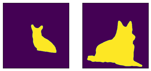
函数 make_grid() 可用于创建表示多个图像网格的张量。此工具函数需要一个 dtype 为 uint8 的单张图像作为输入。

from torchvision.utils import make_grid
from torchvision.io import decode_image
from pathlib import Path

dog1_int = decode_image(str(Path('../assets') / 'dog1.jpg'))
dog2_int = decode_image(str(Path('../assets') / 'dog2.jpg'))
dog_list = [dog1_int, dog2_int]

grid = make_grid(dog_list)
show(grid)

可视化边界框

我们可以使用 draw_bounding_boxes() 在图像上绘制框。我们可以设置颜色、标签、宽度以及字体和字体大小。框的格式为 (xmin, ymin, xmax, ymax)。

from torchvision.utils import draw_bounding_boxes


boxes = torch.tensor([[50, 50, 100, 200], [210, 150, 350, 430]], dtype=torch.float)
colors = ["blue", "yellow"]
result = draw_bounding_boxes(dog1_int, boxes, colors=colors, width=5)
show(result)

自然地，我们也可以绘制 torchvision 检测模型产生的边界框。这里是一个使用从 fasterrcnn_resnet50_fpn() 模型加载的 Faster R-CNN 模型的演示。有关此类模型输出的更多详细信息，您可以参考 实例分割模型。

from torchvision.models.detection import fasterrcnn_resnet50_fpn, FasterRCNN_ResNet50_FPN_Weights


weights = FasterRCNN_ResNet50_FPN_Weights.DEFAULT
transforms = weights.transforms()

images = [transforms(d) for d in dog_list]

model = fasterrcnn_resnet50_fpn(weights=weights, progress=False)
model = model.eval()

outputs = model(images)
print(outputs)

[{'boxes': tensor([[215.9767, 171.1661, 402.0078, 378.7391],
        [344.6341, 172.6735, 357.6114, 220.1435],
        [153.1306, 185.5567, 172.9223, 254.7014]], grad_fn=<StackBackward0>), 'labels': tensor([18,  1,  1]), 'scores': tensor([0.9989, 0.0701, 0.0611], grad_fn=<IndexBackward0>)}, {'boxes': tensor([[ 23.5964, 132.4331, 449.9359, 493.0222],
        [225.8182, 124.6292, 467.2861, 492.2621],
        [ 18.5248, 135.4171, 420.9786, 479.2225]], grad_fn=<StackBackward0>), 'labels': tensor([18, 18, 17]), 'scores': tensor([0.9980, 0.0879, 0.0671], grad_fn=<IndexBackward0>)}]

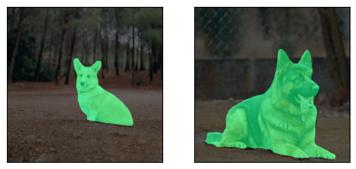
让我们绘制模型检测到的框。我们只会绘制分数高于给定阈值的框。

score_threshold = .8
dogs_with_boxes = [
    draw_bounding_boxes(dog_int, boxes=output['boxes'][output['scores'] > score_threshold], width=4)
    for dog_int, output in zip(dog_list, outputs)
]
show(dogs_with_boxes)

可视化分割掩码

函数 draw_segmentation_masks() 可用于在图像上绘制分割掩码。语义分割模型和实例分割模型的输出不同，因此我们将分别处理它们。

语义分割模型

我们将看到如何将其与使用 fcn_resnet50() 加载的 torchvision 的 FCN Resnet-50 一起使用。首先让我们看一下模型的输出。

from torchvision.models.segmentation import fcn_resnet50, FCN_ResNet50_Weights

weights = FCN_ResNet50_Weights.DEFAULT
transforms = weights.transforms(resize_size=None)

model = fcn_resnet50(weights=weights, progress=False)
model = model.eval()

batch = torch.stack([transforms(d) for d in dog_list])
output = model(batch)['out']
print(output.shape, output.min().item(), output.max().item())

Downloading: "https://download.pytorch.org/models/fcn_resnet50_coco-1167a1af.pth" to /root/.cache/torch/hub/checkpoints/fcn_resnet50_coco-1167a1af.pth
torch.Size([2, 21, 500, 500]) -7.089669704437256 14.858257293701172

如上所示，分割模型的输出是形状为 (batch_size, num_classes, H, W) 的张量。每个值都是一个未归一化的分数，我们可以通过使用 softmax 将它们归一化到 [0, 1]。在 softmax 之后，我们可以将每个值解释为一个概率，表示给定像素属于给定类别的可能性有多大。

让我们绘制检测到的狗类别和船类别的掩码

sem_class_to_idx = {cls: idx for (idx, cls) in enumerate(weights.meta["categories"])}

normalized_masks = torch.nn.functional.softmax(output, dim=1)

dog_and_boat_masks = [
    normalized_masks[img_idx, sem_class_to_idx[cls]]
    for img_idx in range(len(dog_list))
    for cls in ('dog', 'boat')
]

show(dog_and_boat_masks)

正如预期的那样，模型对狗类别很自信，但对船类别则不太自信。

函数 draw_segmentation_masks() 可用于在原始图像上方绘制这些掩码。此函数期望掩码是布尔掩码，但我们上面的掩码包含 [0, 1] 范围内的概率。要获得布尔掩码，我们可以执行以下操作

class_dim = 1
boolean_dog_masks = (normalized_masks.argmax(class_dim) == sem_class_to_idx['dog'])
print(f"shape = {boolean_dog_masks.shape}, dtype = {boolean_dog_masks.dtype}")
show([m.float() for m in boolean_dog_masks])

shape = torch.Size([2, 500, 500]), dtype = torch.bool

上面定义 boolean_dog_masks 的那行代码有点晦涩难懂，但您可以将其理解为以下查询：“哪些像素最有可能属于‘狗’类别？”

注意

虽然我们在这里使用了 normalized_masks，但直接使用模型的未归一化分数也会得到相同的结果（因为 softmax 操作保留了顺序）。

现在我们有了布尔掩码，可以将它们与 draw_segmentation_masks() 一起使用，在原始图像上方绘制它们

from torchvision.utils import draw_segmentation_masks

dogs_with_masks = [
    draw_segmentation_masks(img, masks=mask, alpha=0.7)
    for img, mask in zip(dog_list, boolean_dog_masks)
]
show(dogs_with_masks)

我们可以为每张图像绘制多个掩码！记住，模型返回的掩码数量与类别数量相同。让我们提出与上面相同的查询，但这次是针对所有类别，而不仅仅是狗类别：“对于每个像素和每个类别 C，类别 C 是最有可能的类别吗？”

这个过程有点复杂，所以我们首先演示如何处理单张图像，然后再推广到整个批次。

num_classes = normalized_masks.shape[1]
dog1_masks = normalized_masks[0]
class_dim = 0
dog1_all_classes_masks = dog1_masks.argmax(class_dim) == torch.arange(num_classes)[:, None, None]

print(f"dog1_masks shape = {dog1_masks.shape}, dtype = {dog1_masks.dtype}")
print(f"dog1_all_classes_masks = {dog1_all_classes_masks.shape}, dtype = {dog1_all_classes_masks.dtype}")

dog_with_all_masks = draw_segmentation_masks(dog1_int, masks=dog1_all_classes_masks, alpha=.6)
show(dog_with_all_masks)

dog1_masks shape = torch.Size([21, 500, 500]), dtype = torch.float32
dog1_all_classes_masks = torch.Size([21, 500, 500]), dtype = torch.bool

从上面的图像中我们可以看到，只绘制了 2 个掩码：背景的掩码和狗的掩码。这是因为模型认为在所有像素中，只有这两个类别是最有可能的。如果模型在其他像素中检测到另一个类别是最有可能的，我们就会在上面看到它的掩码。

移除背景掩码很简单，只需传递 masks=dog1_all_classes_masks[1:] 即可，因为背景类别是索引为 0 的类别。

现在让我们对整个图像批次做同样的处理。代码类似，但涉及更多关于维度的操作。

class_dim = 1
all_classes_masks = normalized_masks.argmax(class_dim) == torch.arange(num_classes)[:, None, None, None]
print(f"shape = {all_classes_masks.shape}, dtype = {all_classes_masks.dtype}")
# The first dimension is the classes now, so we need to swap it
all_classes_masks = all_classes_masks.swapaxes(0, 1)

dogs_with_masks = [
    draw_segmentation_masks(img, masks=mask, alpha=.6)
    for img, mask in zip(dog_list, all_classes_masks)
]
show(dogs_with_masks)

shape = torch.Size([21, 2, 500, 500]), dtype = torch.bool

实例分割模型

实例分割模型与语义分割模型的输出显著不同。我们将在这里看到如何绘制这类模型的掩码。首先让我们分析 Mask-RCNN 模型的输出。请注意，这些模型不需要图像归一化，因此我们不需要使用归一化的批次。

注意

我们将在这里描述 Mask-RCNN 模型的输出。目标检测、实例分割和人体关键点检测 中的模型都具有相似的输出格式，但其中一些可能包含额外信息，例如 keypointrcnn_resnet50_fpn() 的关键点，而有些可能不包含掩码，例如 fasterrcnn_resnet50_fpn()。

from torchvision.models.detection import maskrcnn_resnet50_fpn, MaskRCNN_ResNet50_FPN_Weights

weights = MaskRCNN_ResNet50_FPN_Weights.DEFAULT
transforms = weights.transforms()

images = [transforms(d) for d in dog_list]

model = maskrcnn_resnet50_fpn(weights=weights, progress=False)
model = model.eval()

output = model(images)
print(output)

Downloading: "https://download.pytorch.org/models/maskrcnn_resnet50_fpn_coco-bf2d0c1e.pth" to /root/.cache/torch/hub/checkpoints/maskrcnn_resnet50_fpn_coco-bf2d0c1e.pth
[{'boxes': tensor([[219.7444, 168.1722, 400.7378, 384.0263],
        [343.9716, 171.2287, 358.3447, 222.6263],
        [301.0303, 192.6917, 313.8879, 232.3154]], grad_fn=<StackBackward0>), 'labels': tensor([18,  1,  1]), 'scores': tensor([0.9987, 0.7187, 0.6525], grad_fn=<IndexBackward0>), 'masks': tensor([[[[0., 0., 0.,  ..., 0., 0., 0.],
          [0., 0., 0.,  ..., 0., 0., 0.],
          [0., 0., 0.,  ..., 0., 0., 0.],
          ...,
          [0., 0., 0.,  ..., 0., 0., 0.],
          [0., 0., 0.,  ..., 0., 0., 0.],
          [0., 0., 0.,  ..., 0., 0., 0.]]],


        [[[0., 0., 0.,  ..., 0., 0., 0.],
          [0., 0., 0.,  ..., 0., 0., 0.],
          [0., 0., 0.,  ..., 0., 0., 0.],
          ...,
          [0., 0., 0.,  ..., 0., 0., 0.],
          [0., 0., 0.,  ..., 0., 0., 0.],
          [0., 0., 0.,  ..., 0., 0., 0.]]],


        [[[0., 0., 0.,  ..., 0., 0., 0.],
          [0., 0., 0.,  ..., 0., 0., 0.],
          [0., 0., 0.,  ..., 0., 0., 0.],
          ...,
          [0., 0., 0.,  ..., 0., 0., 0.],
          [0., 0., 0.,  ..., 0., 0., 0.],
          [0., 0., 0.,  ..., 0., 0., 0.]]]], grad_fn=<UnsqueezeBackward0>)}, {'boxes': tensor([[ 44.6767, 137.9018, 446.5324, 487.3429],
        [  0.0000, 288.0053, 489.9292, 490.2352]], grad_fn=<StackBackward0>), 'labels': tensor([18, 15]), 'scores': tensor([0.9978, 0.0697], grad_fn=<IndexBackward0>), 'masks': tensor([[[[0., 0., 0.,  ..., 0., 0., 0.],
          [0., 0., 0.,  ..., 0., 0., 0.],
          [0., 0., 0.,  ..., 0., 0., 0.],
          ...,
          [0., 0., 0.,  ..., 0., 0., 0.],
          [0., 0., 0.,  ..., 0., 0., 0.],
          [0., 0., 0.,  ..., 0., 0., 0.]]],


        [[[0., 0., 0.,  ..., 0., 0., 0.],
          [0., 0., 0.,  ..., 0., 0., 0.],
          [0., 0., 0.,  ..., 0., 0., 0.],
          ...,
          [0., 0., 0.,  ..., 0., 0., 0.],
          [0., 0., 0.,  ..., 0., 0., 0.],
          [0., 0., 0.,  ..., 0., 0., 0.]]]], grad_fn=<UnsqueezeBackward0>)}]

让我们分解一下。对于批次中的每张图像，模型会输出一些检测结果（或实例）。每张输入图像的检测数量各不相同。每个实例都由其边界框、标签、分数和掩码描述。

输出的组织方式如下：输出是一个长度为 batch_size 的列表。列表中的每个条目对应一张输入图像，它是一个字典，包含键‘boxes’、‘labels’、‘scores’和‘masks’。与这些键关联的每个值都包含 num_instances 个元素。在上面的例子中，第一张图像检测到 3 个实例，第二张检测到 2 个实例。

如上所述，可以使用 draw_bounding_boxes() 绘制边界框，但在这里我们更关注掩码。这些掩码与我们在上面看到的语义分割模型的掩码截然不同。

dog1_output = output[0]
dog1_masks = dog1_output['masks']
print(f"shape = {dog1_masks.shape}, dtype = {dog1_masks.dtype}, "
      f"min = {dog1_masks.min()}, max = {dog1_masks.max()}")

shape = torch.Size([3, 1, 500, 500]), dtype = torch.float32, min = 0.0, max = 0.9999862909317017

这里的掩码对应于概率，指示每个像素属于该实例预测标签的可能性。这些预测标签对应于同一输出字典中的‘labels’元素。让我们看看第一张图像的实例预测了哪些标签。

print("For the first dog, the following instances were detected:")
print([weights.meta["categories"][label] for label in dog1_output['labels']])

For the first dog, the following instances were detected:
['dog', 'person', 'person']

有趣的是，模型在图像中检测到两个人。让我们继续绘制这些掩码。draw_segmentation_masks() 函数需要布尔掩码，因此我们需要将这些概率转换为布尔值。记住，这些掩码的语义是“此像素属于预测类别的可能性有多大？”。因此，将这些掩码转换为布尔值的一个自然方法是使用 0.5 的概率进行阈值处理（也可以选择不同的阈值）。

proba_threshold = 0.5
dog1_bool_masks = dog1_output['masks'] > proba_threshold
print(f"shape = {dog1_bool_masks.shape}, dtype = {dog1_bool_masks.dtype}")

# There's an extra dimension (1) to the masks. We need to remove it
dog1_bool_masks = dog1_bool_masks.squeeze(1)

show(draw_segmentation_masks(dog1_int, dog1_bool_masks, alpha=0.9))

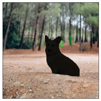
shape = torch.Size([3, 1, 500, 500]), dtype = torch.bool

模型似乎正确地检测到了狗，但也将树木误认为是人。更仔细地查看分数将有助于我们绘制更相关的掩码。

print(dog1_output['scores'])

tensor([0.9987, 0.7187, 0.6525], grad_fn=<IndexBackward0>)

显然，模型对狗的检测比对人的检测更有信心。这是个好消息。在绘制掩码时，我们可以只选择得分较高的掩码。这里我们使用 0.75 的分数阈值，并绘制第二只狗的掩码。

score_threshold = .75

boolean_masks = [
    out['masks'][out['scores'] > score_threshold] > proba_threshold
    for out in output
]

dogs_with_masks = [
    draw_segmentation_masks(img, mask.squeeze(1))
    for img, mask in zip(dog_list, boolean_masks)
]
show(dogs_with_masks)

第一张图像中的两个‘人’的掩码未被选中，因为它们的得分低于分数阈值。类似地，在第二张图像中，类别为 15（对应‘长凳’）的实例也未被选中。

可视化关键点

函数 draw_keypoints() 可用于在图像上绘制关键点。我们将看到如何将其与使用 keypointrcnn_resnet50_fpn() 加载的 torchvision 的 KeypointRCNN 一起使用。我们首先将查看模型的输出。

from torchvision.models.detection import keypointrcnn_resnet50_fpn, KeypointRCNN_ResNet50_FPN_Weights
from torchvision.io import decode_image

person_int = decode_image(str(Path("../assets") / "person1.jpg"))

weights = KeypointRCNN_ResNet50_FPN_Weights.DEFAULT
transforms = weights.transforms()

person_float = transforms(person_int)

model = keypointrcnn_resnet50_fpn(weights=weights, progress=False)
model = model.eval()

outputs = model([person_float])
print(outputs)

Downloading: "https://download.pytorch.org/models/keypointrcnn_resnet50_fpn_coco-fc266e95.pth" to /root/.cache/torch/hub/checkpoints/keypointrcnn_resnet50_fpn_coco-fc266e95.pth
[{'boxes': tensor([[124.3751, 177.9242, 327.6354, 574.7064],
        [124.3625, 180.7574, 290.1061, 390.7958]], grad_fn=<StackBackward0>), 'labels': tensor([1, 1]), 'scores': tensor([0.9998, 0.1070], grad_fn=<IndexBackward0>), 'keypoints': tensor([[[208.0176, 214.2408,   1.0000],
         [208.0176, 207.0375,   1.0000],
         [197.8246, 210.6392,   1.0000],
         [208.0176, 211.8398,   1.0000],
         [178.6378, 217.8425,   1.0000],
         [221.2086, 253.8590,   1.0000],
         [160.6502, 269.4662,   1.0000],
         [243.9929, 304.2822,   1.0000],
         [138.4654, 328.8935,   1.0000],
         [277.5698, 340.8990,   1.0000],
         [153.4551, 374.5144,   1.0000],
         [226.0053, 375.7150,   1.0000],
         [226.0053, 370.3125,   1.0000],
         [221.8082, 455.5516,   1.0000],
         [273.9723, 448.9486,   1.0000],
         [193.6275, 546.1932,   1.0000],
         [273.3727, 545.5930,   1.0000]],

        [[207.8327, 214.6636,   1.0000],
         [207.2343, 207.4622,   1.0000],
         [198.2590, 209.8627,   1.0000],
         [208.4310, 210.4628,   1.0000],
         [178.5134, 218.2642,   1.0000],
         [219.7997, 251.8704,   1.0000],
         [162.3579, 269.2736,   1.0000],
         [245.5289, 304.6800,   1.0000],
         [138.4238, 330.4848,   1.0000],
         [278.4382, 346.0876,   1.0000],
         [153.3826, 374.8929,   1.0000],
         [233.5618, 368.2917,   1.0000],
         [225.7832, 367.6916,   1.0000],
         [289.8069, 357.4897,   1.0000],
         [245.5289, 389.8956,   1.0000],
         [281.4300, 349.0882,   1.0000],
         [209.0294, 389.8956,   1.0000]]], grad_fn=<CopySlices>), 'keypoints_scores': tensor([[16.0163, 16.6672, 15.8312,  4.6510, 14.2053,  8.8280,  9.1136, 12.2084,
         12.1901, 13.8453, 10.7090,  5.5852,  7.5005, 11.3378,  9.3700,  8.2987,
          8.4479],
        [12.9326, 13.8158, 14.9053,  3.9368, 12.9585,  6.4240,  6.8328, 10.4227,
          9.2907, 10.1066, 10.1019,  0.1822,  4.3057, -4.9904, -2.7409, -2.7874,
         -3.9329]], grad_fn=<CopySlices>)}]

如我们所见，输出包含一个字典列表。输出列表的长度为 batch_size。我们目前只有一张图像，因此列表长度为 1。列表中的每个条目对应一张输入图像，它是一个字典，包含键 boxes、labels、scores、keypoints 和 keypoint_scores。与这些键关联的每个值都包含 num_instances 个元素。在上面的例子中，图像中检测到 2 个实例。

kpts = outputs[0]['keypoints']
scores = outputs[0]['scores']

print(kpts)
print(scores)

tensor([[[208.0176, 214.2408,   1.0000],
         [208.0176, 207.0375,   1.0000],
         [197.8246, 210.6392,   1.0000],
         [208.0176, 211.8398,   1.0000],
         [178.6378, 217.8425,   1.0000],
         [221.2086, 253.8590,   1.0000],
         [160.6502, 269.4662,   1.0000],
         [243.9929, 304.2822,   1.0000],
         [138.4654, 328.8935,   1.0000],
         [277.5698, 340.8990,   1.0000],
         [153.4551, 374.5144,   1.0000],
         [226.0053, 375.7150,   1.0000],
         [226.0053, 370.3125,   1.0000],
         [221.8082, 455.5516,   1.0000],
         [273.9723, 448.9486,   1.0000],
         [193.6275, 546.1932,   1.0000],
         [273.3727, 545.5930,   1.0000]],

        [[207.8327, 214.6636,   1.0000],
         [207.2343, 207.4622,   1.0000],
         [198.2590, 209.8627,   1.0000],
         [208.4310, 210.4628,   1.0000],
         [178.5134, 218.2642,   1.0000],
         [219.7997, 251.8704,   1.0000],
         [162.3579, 269.2736,   1.0000],
         [245.5289, 304.6800,   1.0000],
         [138.4238, 330.4848,   1.0000],
         [278.4382, 346.0876,   1.0000],
         [153.3826, 374.8929,   1.0000],
         [233.5618, 368.2917,   1.0000],
         [225.7832, 367.6916,   1.0000],
         [289.8069, 357.4897,   1.0000],
         [245.5289, 389.8956,   1.0000],
         [281.4300, 349.0882,   1.0000],
         [209.0294, 389.8956,   1.0000]]], grad_fn=<CopySlices>)
tensor([0.9998, 0.1070], grad_fn=<IndexBackward0>)

KeypointRCNN 模型检测到图像中有两个实例。如果使用 draw_bounding_boxes() 绘制边界框，您会认出它们是人和冲浪板。如果我们查看分数，就会发现模型对人的检测比对冲浪板的检测更有信心。现在我们可以设置一个置信度阈值，并绘制我们足够自信的实例。让我们设置一个 0.75 的阈值，并过滤出对应于人的关键点。

detect_threshold = 0.75
idx = torch.where(scores > detect_threshold)
keypoints = kpts[idx]

print(keypoints)

tensor([[[208.0176, 214.2408,   1.0000],
         [208.0176, 207.0375,   1.0000],
         [197.8246, 210.6392,   1.0000],
         [208.0176, 211.8398,   1.0000],
         [178.6378, 217.8425,   1.0000],
         [221.2086, 253.8590,   1.0000],
         [160.6502, 269.4662,   1.0000],
         [243.9929, 304.2822,   1.0000],
         [138.4654, 328.8935,   1.0000],
         [277.5698, 340.8990,   1.0000],
         [153.4551, 374.5144,   1.0000],
         [226.0053, 375.7150,   1.0000],
         [226.0053, 370.3125,   1.0000],
         [221.8082, 455.5516,   1.0000],
         [273.9723, 448.9486,   1.0000],
         [193.6275, 546.1932,   1.0000],
         [273.3727, 545.5930,   1.0000]]], grad_fn=<IndexBackward0>)

太好了，现在我们有了对应于人的关键点。每个关键点由 x, y 坐标和可见性表示。现在我们可以使用 draw_keypoints() 函数绘制关键点。注意，该工具函数需要 uint8 图像。

from torchvision.utils import draw_keypoints

res = draw_keypoints(person_int, keypoints, colors="blue", radius=3)
show(res)

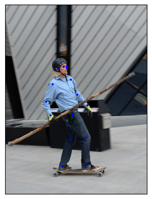
正如我们所见，关键点在图像上方显示为彩色圆圈。一个人的 coco 关键点是有序的，表示以下列表。

coco_keypoints = [
    "nose", "left_eye", "right_eye", "left_ear", "right_ear",
    "left_shoulder", "right_shoulder", "left_elbow", "right_elbow",
    "left_wrist", "right_wrist", "left_hip", "right_hip",
    "left_knee", "right_knee", "left_ankle", "right_ankle",
]

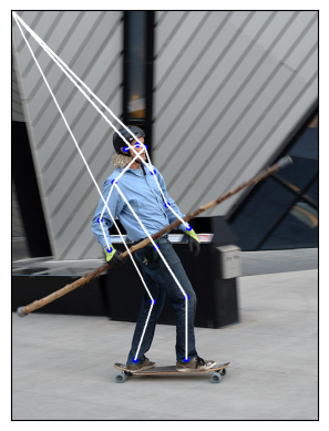
如果我们有兴趣连接关键点怎么办？这在创建姿态检测或行为识别时特别有用。我们可以使用 connectivity 参数轻松连接关键点。仔细观察会发现，我们需要按以下顺序连接点以构建人体骨骼。

鼻子 -> 左眼 -> 左耳。(0, 1), (1, 3)

鼻子 -> 右眼 -> 右耳。(0, 2), (2, 4)

鼻子 -> 左肩 -> 左肘 -> 左腕。(0, 5), (5, 7), (7, 9)

鼻子 -> 右肩 -> 右肘 -> 右腕。(0, 6), (6, 8), (8, 10)

左肩 -> 左臀 -> 左膝 -> 左踝。(5, 11), (11, 13), (13, 15)

右肩 -> 右臀 -> 右膝 -> 右踝。(6, 12), (12, 14), (14, 16)

我们将创建一个包含这些要连接的关键点 ID 的列表。

connect_skeleton = [
    (0, 1), (0, 2), (1, 3), (2, 4), (0, 5), (0, 6), (5, 7), (6, 8),
    (7, 9), (8, 10), (5, 11), (6, 12), (11, 13), (12, 14), (13, 15), (14, 16)
]

我们将上面的列表传递给 connectivity 参数来连接关键点。

res = draw_keypoints(person_int, keypoints, connectivity=connect_skeleton, colors="blue", radius=4, width=3)
show(res)

看起来相当不错。

绘制带有可见性的关键点

让我们看看另一个关键点预测模块产生的结果，并显示连接性

prediction = torch.tensor(
    [[[208.0176, 214.2409, 1.0000],
      [000.0000, 000.0000, 0.0000],
      [197.8246, 210.6392, 1.0000],
      [000.0000, 000.0000, 0.0000],
      [178.6378, 217.8425, 1.0000],
      [221.2086, 253.8591, 1.0000],
      [160.6502, 269.4662, 1.0000],
      [243.9929, 304.2822, 1.0000],
      [138.4654, 328.8935, 1.0000],
      [277.5698, 340.8990, 1.0000],
      [153.4551, 374.5145, 1.0000],
      [000.0000, 000.0000, 0.0000],
      [226.0053, 370.3125, 1.0000],
      [221.8081, 455.5516, 1.0000],
      [273.9723, 448.9486, 1.0000],
      [193.6275, 546.1933, 1.0000],
      [273.3727, 545.5930, 1.0000]]]
)

res = draw_keypoints(person_int, prediction, connectivity=connect_skeleton, colors="blue", radius=4, width=3)
show(res)

那里发生了什么？预测新关键点的模型无法检测到滑板运动员左上方身体上隐藏的三个点。更准确地说，模型预测左眼、左耳和左臀的关键点为 (x, y, vis) = (0, 0, 0)。所以我们肯定不想显示这些关键点和连接，而且你也不必这样做。查看 draw_keypoints() 的参数，我们可以看到可以将一个可见性张量作为附加参数传递。根据模型的预测，可见性是关键点的第三个维度，我们只需将其提取出来即可。让我们将 prediction 分割成关键点坐标和它们各自的可见性，并将它们都作为参数传递给 draw_keypoints()。

coordinates, visibility = prediction.split([2, 1], dim=-1)
visibility = visibility.bool()

res = draw_keypoints(
    person_int, coordinates, visibility=visibility, connectivity=connect_skeleton, colors="blue", radius=4, width=3
)
show(res)

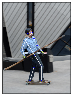
我们可以看到未检测到的关键点没有被绘制出来，并且跳过了不可见的关键点连接。这可以减少多重检测图像上的噪声，或者像我们这样的情况，关键点预测模型遗漏了一些检测。大多数 torch 关键点预测模型会返回每个预测的可见性，您可以直接使用。我们在第一个例子中使用的 keypointrcnn_resnet50_fpn() 模型也是如此。