使用 ONNX 将模型从 PyTorch 传输到 Caffe2 和移动设备

在本教程中，我们将介绍如何使用 ONNX 将 PyTorch 中定义的模型转换为 ONNX 格式，然后将其加载到 Caffe2 中。进入 Caffe2 后，我们可以运行模型以仔细检查它是否已正确导出，然后我们将展示如何使用 Caffe2 功能（例如移动导出器）在移动设备上执行模型。

对于本教程，您需要安装 onnx 和 Caffe2。您可以使用 pip install onnx 获取 onnx 的二进制版本。

注意：本教程需要 PyTorch master 分支，可以按照 此处 的说明进行安装

# Some standard imports
import io
import numpy as np

from torch import nn
import torch.utils.model_zoo as model_zoo
import torch.onnx

超分辨率是一种提高图像、视频分辨率的方法，广泛应用于图像处理或视频编辑。在本教程中，我们将首先使用一个带有虚拟输入的小型超分辨率模型。

首先，让我们在 PyTorch 中创建一个 SuperResolution 模型。 该模型 直接来自 PyTorch 的示例，未经修改

# Super Resolution model definition in PyTorch
import torch.nn as nn
import torch.nn.init as init


class SuperResolutionNet(nn.Module):
    def __init__(self, upscale_factor, inplace=False):
        super(SuperResolutionNet, self).__init__()

        self.relu = nn.ReLU(inplace=inplace)
        self.conv1 = nn.Conv2d(1, 64, (5, 5), (1, 1), (2, 2))
        self.conv2 = nn.Conv2d(64, 64, (3, 3), (1, 1), (1, 1))
        self.conv3 = nn.Conv2d(64, 32, (3, 3), (1, 1), (1, 1))
        self.conv4 = nn.Conv2d(32, upscale_factor ** 2, (3, 3), (1, 1), (1, 1))
        self.pixel_shuffle = nn.PixelShuffle(upscale_factor)

        self._initialize_weights()

    def forward(self, x):
        x = self.relu(self.conv1(x))
        x = self.relu(self.conv2(x))
        x = self.relu(self.conv3(x))
        x = self.pixel_shuffle(self.conv4(x))
        return x

    def _initialize_weights(self):
        init.orthogonal_(self.conv1.weight, init.calculate_gain('relu'))
        init.orthogonal_(self.conv2.weight, init.calculate_gain('relu'))
        init.orthogonal_(self.conv3.weight, init.calculate_gain('relu'))
        init.orthogonal_(self.conv4.weight)

# Create the super-resolution model by using the above model definition.
torch_model = SuperResolutionNet(upscale_factor=3)

通常，您现在将训练此模型；但是，在本教程中，我们将改为下载一些预先训练的权重。请注意，此模型没有经过充分训练以获得良好的准确性，此处仅用于演示目的。

# Load pretrained model weights
model_url = 'https://s3.amazonaws.com/pytorch/test_data/export/superres_epoch100-44c6958e.pth'
batch_size = 1    # just a random number

# Initialize model with the pretrained weights
map_location = lambda storage, loc: storage
if torch.cuda.is_available():
    map_location = None
torch_model.load_state_dict(model_zoo.load_url(model_url, map_location=map_location))

# set the train mode to false since we will only run the forward pass.
torch_model.train(False)

在 PyTorch 中导出模型通过跟踪进行。要导出模型，请调用 torch.onnx._export() 函数。这将执行模型，记录用于计算输出的操作符的跟踪。因为 _export 会运行模型，所以我们需要提供一个输入张量 x。此张量中的值并不重要；只要大小合适，它可以是图像或随机张量。

要了解有关 PyTorch 导出接口的更多详细信息，请查看 torch.onnx 文档。

# Input to the model
x = torch.randn(batch_size, 1, 224, 224, requires_grad=True)

# Export the model
torch_out = torch.onnx._export(torch_model,             # model being run
                               x,                       # model input (or a tuple for multiple inputs)
                               "super_resolution.onnx", # where to save the model (can be a file or file-like object)
                               export_params=True)      # store the trained parameter weights inside the model file

torch_out 是执行模型后的输出。通常您可以忽略此输出，但在这里我们将使用它来验证我们导出的模型在 Caffe2 中运行时是否计算出相同的值。

现在让我们采用 ONNX 表示并在 Caffe2 中使用它。这部分通常可以在单独的进程或另一台机器上完成，但我们将继续在同一个进程中进行，以便我们可以验证 Caffe2 和 PyTorch 是否为网络计算相同的值

import onnx
import caffe2.python.onnx.backend as onnx_caffe2_backend

# Load the ONNX ModelProto object. model is a standard Python protobuf object
model = onnx.load("super_resolution.onnx")

# prepare the caffe2 backend for executing the model this converts the ONNX model into a
# Caffe2 NetDef that can execute it. Other ONNX backends, like one for CNTK will be
# availiable soon.
prepared_backend = onnx_caffe2_backend.prepare(model)

# run the model in Caffe2

# Construct a map from input names to Tensor data.
# The graph of the model itself contains inputs for all weight parameters, after the input image.
# Since the weights are already embedded, we just need to pass the input image.
# Set the first input.
W = {model.graph.input[0].name: x.data.numpy()}

# Run the Caffe2 net:
c2_out = prepared_backend.run(W)[0]

# Verify the numerical correctness upto 3 decimal places
np.testing.assert_almost_equal(torch_out.data.cpu().numpy(), c2_out, decimal=3)

print("Exported model has been executed on Caffe2 backend, and the result looks good!")

我们应该看到 PyTorch 和 Caffe2 运行的输出在数值上匹配到小数点后 3 位。附带说明一下，如果它们不匹配，则说明 Caffe2 和 PyTorch 中的操作符实现方式不同，在这种情况下请联系我们。

使用 ONNX 传输 SRResNet

使用与上述相同的流程，我们还传输了一个有趣的新模型“SRResNet”，用于 这篇论文 中提出的超分辨率（感谢 Twitter 的作者为本教程提供了代码和预训练参数）。模型定义和预训练模型可以在 此处 找到。以下是 SRResNet 模型输入、输出的样子。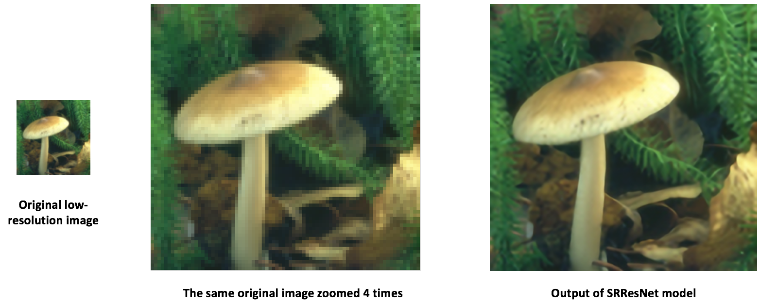

在移动设备上运行模型

到目前为止，我们已经从 PyTorch 导出了一个模型，并展示了如何在 Caffe2 中加载和运行它。现在模型已加载到 Caffe2 中，我们可以将其转换为适合 在移动设备上运行 的格式。

我们将使用 Caffe2 的 mobile_exporter 来生成可以在移动设备上运行的两个模型 protobuf。第一个用于使用正确的权重初始化网络，第二个用于实际运行执行模型。在本教程的其余部分，我们将继续使用小型超分辨率模型。

# extract the workspace and the model proto from the internal representation
c2_workspace = prepared_backend.workspace
c2_model = prepared_backend.predict_net

# Now import the caffe2 mobile exporter
from caffe2.python.predictor import mobile_exporter

# call the Export to get the predict_net, init_net. These nets are needed for running things on mobile
init_net, predict_net = mobile_exporter.Export(c2_workspace, c2_model, c2_model.external_input)

# Let's also save the init_net and predict_net to a file that we will later use for running them on mobile
with open('init_net.pb', "wb") as fopen:
    fopen.write(init_net.SerializeToString())
with open('predict_net.pb', "wb") as fopen:
    fopen.write(predict_net.SerializeToString())

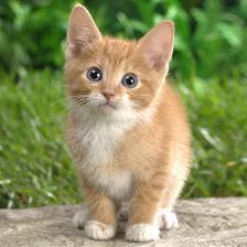
init_net 中嵌入了模型参数和模型输入，predict_net 将用于在运行时指导 init_net 的执行。在本教程中，我们将使用上面生成的 init_net 和 predict_net，并在普通的 Caffe2 后端和移动设备上运行它们，并验证两次运行中产生的输出高分辨率猫图像是否相同。

在本教程中，我们将使用一张广泛使用的著名猫图像，如下所示

# Some standard imports
from caffe2.proto import caffe2_pb2
from caffe2.python import core, net_drawer, net_printer, visualize, workspace, utils

import numpy as np
import os
import subprocess
from PIL import Image
from matplotlib import pyplot
from skimage import io, transform

首先，让我们加载图像，使用标准的 skimage python 库对其进行预处理。请注意，这种预处理是处理用于训练/测试神经网络数据的标准做法。

# load the image
img_in = io.imread("./_static/img/cat.jpg")

# resize the image to dimensions 224x224
img = transform.resize(img_in, [224, 224])

# save this resized image to be used as input to the model
io.imsave("./_static/img/cat_224x224.jpg", img)

现在，下一步，让我们获取调整大小后的猫图像，并在 Caffe2 后端运行超分辨率模型，并保存输出图像。以下图像处理步骤已从 PyTorch 超分辨率模型的实现中采用，此处

# load the resized image and convert it to Ybr format
img = Image.open("./_static/img/cat_224x224.jpg")
img_ycbcr = img.convert('YCbCr')
img_y, img_cb, img_cr = img_ycbcr.split()

# Let's run the mobile nets that we generated above so that caffe2 workspace is properly initialized
workspace.RunNetOnce(init_net)
workspace.RunNetOnce(predict_net)

# Caffe2 has a nice net_printer to be able to inspect what the net looks like and identify
# what our input and output blob names are.
print(net_printer.to_string(predict_net))

从上面的输出中，我们可以看到输入名为“9”，输出名为“27”（我们使用数字作为 blob 名称有点奇怪，但这是因为跟踪 JIT 为模型生成了编号条目）

# Now, let's also pass in the resized cat image for processing by the model.
workspace.FeedBlob("9", np.array(img_y)[np.newaxis, np.newaxis, :, :].astype(np.float32))

# run the predict_net to get the model output
workspace.RunNetOnce(predict_net)

# Now let's get the model output blob
img_out = workspace.FetchBlob("27")

现在，我们将参考 PyTorch 超分辨率模型实现中的后处理步骤，此处，以构建最终的输出图像并保存图像。

img_out_y = Image.fromarray(np.uint8((img_out[0, 0]).clip(0, 255)), mode='L')

# get the output image follow post-processing step from PyTorch implementation
final_img = Image.merge(
    "YCbCr", [
        img_out_y,
        img_cb.resize(img_out_y.size, Image.BICUBIC),
        img_cr.resize(img_out_y.size, Image.BICUBIC),
    ]).convert("RGB")

# Save the image, we will compare this with the output image from mobile device
final_img.save("./_static/img/cat_superres.jpg")

我们已经在纯 Caffe2 后端完成了移动网络的运行，现在，让我们在 Android 设备上执行模型并获取模型输出。

注意：对于 Android 开发，需要 adb shell，否则本教程的以下部分将无法运行。

在我们在移动设备上运行模型的第一步中，我们将推送一个用于移动设备的原生速度基准测试二进制文件到 adb。该二进制文件可以在移动设备上执行模型，还可以导出我们稍后可以检索的模型输出。该二进制文件可以在 此处 获得。要构建二进制文件，请按照 此处 的说明执行 build_android.sh 脚本。

注意：您需要安装 ANDROID_NDK 并设置环境变量 ANDROID_NDK=ndk 根目录的路径

# let's first push a bunch of stuff to adb, specify the path for the binary
CAFFE2_MOBILE_BINARY = ('caffe2/binaries/speed_benchmark')

# we had saved our init_net and proto_net in steps above, we use them now.
# Push the binary and the model protos
os.system('adb push ' + CAFFE2_MOBILE_BINARY + ' /data/local/tmp/')
os.system('adb push init_net.pb /data/local/tmp')
os.system('adb push predict_net.pb /data/local/tmp')

# Let's serialize the input image blob to a blob proto and then send it to mobile for execution.
with open("input.blobproto", "wb") as fid:
    fid.write(workspace.SerializeBlob("9"))

# push the input image blob to adb
os.system('adb push input.blobproto /data/local/tmp/')

# Now we run the net on mobile, look at the speed_benchmark --help for what various options mean
os.system(
    'adb shell /data/local/tmp/speed_benchmark '                     # binary to execute
    '--init_net=/data/local/tmp/super_resolution_mobile_init.pb '    # mobile init_net
    '--net=/data/local/tmp/super_resolution_mobile_predict.pb '      # mobile predict_net
    '--input=9 '                                                     # name of our input image blob
    '--input_file=/data/local/tmp/input.blobproto '                  # serialized input image
    '--output_folder=/data/local/tmp '                               # destination folder for saving mobile output
    '--output=27,9 '                                                 # output blobs we are interested in
    '--iter=1 '                                                      # number of net iterations to execute
    '--caffe2_log_level=0 '
)

# get the model output from adb and save to a file
os.system('adb pull /data/local/tmp/27 ./output.blobproto')


# We can recover the output content and post-process the model using same steps as we followed earlier
blob_proto = caffe2_pb2.BlobProto()
blob_proto.ParseFromString(open('./output.blobproto').read())
img_out = utils.Caffe2TensorToNumpyArray(blob_proto.tensor)
img_out_y = Image.fromarray(np.uint8((img_out[0,0]).clip(0, 255)), mode='L')
final_img = Image.merge(
    "YCbCr", [
        img_out_y,
        img_cb.resize(img_out_y.size, Image.BICUBIC),
        img_cr.resize(img_out_y.size, Image.BICUBIC),
    ]).convert("RGB")
final_img.save("./_static/img/cat_superres_mobile.jpg")

现在，您可以比较图像 cat_superres.jpg（纯 caffe2 后端执行的模型输出）和 cat_superres_mobile.jpg（移动执行的模型输出），并查看两张图像是否看起来相同。如果它们看起来不同，则表示在移动设备上的执行出现了问题，在这种情况下，请联系 Caffe2 社区。您应该会看到输出图像如下所示

使用上述步骤，您可以轻松地在移动设备上部署模型。此外，有关 caffe2 移动后端的更多信息，请查看 caffe2-android-demo。