确保输入使用正确的内存格式可以显著影响 PyTorch 视觉模型的运行时间。如有疑问,请选择 Channels Last 内存格式。
在处理接受多媒体(例如图像张量)作为输入的 PyTorch 视觉模型时,张量的内存格式可以显著影响 在使用 CPU 后端和 XNNPACK 的移动平台上模型的推理执行速度。这对于服务器平台上的训练和推理也适用,但对于移动设备和用户而言,延迟尤为关键。
本文大纲
- 深入探讨 C++ 中的矩阵存储/内存表示。介绍 行主序和列主序。
- 按照与存储表示相同或不同的顺序遍历矩阵的影响,并附带一个示例。
- Cachegrind 简介;一个检查代码缓存友好性的工具。
- PyTorch 运算符支持的内存格式。
- 确保使用 XNNPACK 优化高效执行模型的最佳实践示例。
C++ 中的矩阵存储表示
图像以多维张量的形式输入到 PyTorch ML 模型中。这些张量具有特定的内存格式。为了更好地理解这个概念,让我们看看二维矩阵是如何存储在内存中的。
广义上讲,有 2 种主要方式可以高效地在内存中存储多维数据。
- 行主序: 在这种格式中,矩阵按行顺序存储,每行在内存中存储在下一行之前。即,第 N 行在第 N+1 行之前。
- 列主序: 在这种格式中,矩阵按列顺序存储,每列在内存中存储在下一列之前。即,第 N 列在第 N+1 列之前。
您可以在下面的图表中看到差异。
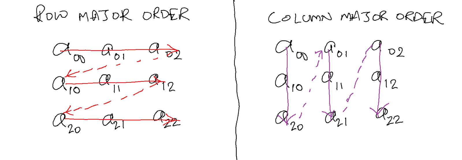
C++ 以行主序格式存储多维数据。
高效访问二维矩阵的元素
与存储格式类似,有 2 种方法可以访问二维矩阵中的数据。
- 首先遍历行: 在处理下一行的任何元素之前,处理一行的所有元素。
- 首先遍历列: 在处理下一列的任何元素之前,处理一列的所有元素。
为了达到最大效率,应始终以与数据存储格式相同的格式访问数据。即,如果数据以行主序存储,则应尝试以该顺序访问它。
下面的代码 (main.cpp) 展示了 2 种方法 访问 4000×4000 二维矩阵的所有元素。
#include <iostream>
#include <chrono>

// loop1 accesses data in matrix 'a' in row major order,
// since i is the outer loop variable, and j is the
// inner loop variable.
int loop1(int a[4000][4000]) {
 int s = 0;
 for (int i = 0; i < 4000; ++i) {
   for (int j = 0; j < 4000; ++j) {
     s += a[i][j];
   }
 }
 return s;
}

// loop2 accesses data in matrix 'a' in column major order
// since j is the outer loop variable, and i is the
// inner loop variable.
int loop2(int a[4000][4000]) {
 int s = 0;
 for (int j = 0; j < 4000; ++j) {
   for (int i = 0; i < 4000; ++i) {
     s += a[i][j];
   }
 }
 return s;
}

int main() {
 static int a[4000][4000] = {0};
 for (int i = 0; i < 100; ++i) {
   int x = rand() % 4000;
   int y = rand() % 4000;
   a[x][y] = rand() % 1000;
 }

 auto start = std::chrono::high_resolution_clock::now();
 auto end = start;
 int s = 0;

#if defined RUN_LOOP1
 start = std::chrono::high_resolution_clock::now();

 s = 0;
 for (int i = 0; i < 10; ++i) {
   s += loop1(a);
   s = s % 100;
 }
 end = std::chrono::high_resolution_clock::now();

 std::cout << "s = " << s << std::endl;
 std::cout << "Time for loop1: "
   << std::chrono::duration<double, std::milli>(end - start).count()
   << "ms" << std::endl;
#endif

#if defined RUN_LOOP2
 start = std::chrono::high_resolution_clock::now();
 s = 0;
 for (int i = 0; i < 10; ++i) {
   s += loop2(a);
   s = s % 100;
 }
 end = std::chrono::high_resolution_clock::now();

 std::cout << "s = " << s << std::endl;
 std::cout << "Time for loop2: "
   << std::chrono::duration<double, std::milli>(end - start).count()
   << "ms" << std::endl;
#endif
}


Let’s build and run this program and see what it prints.

g++ -O2 main.cpp -DRUN_LOOP1 -DRUN_LOOP2
./a.out


Prints the following:

s = 70
Time for loop1: 77.0687ms
s = 70
Time for loop2: 1219.49ms
loop1() 比 loop2() 快 15 倍。为什么会这样?让我们在下面找出答案!
使用 Cachegrind 测量缓存未命中
Cachegrind 是一个缓存分析工具,用于查看程序导致了多少 I1(一级指令)、D1(一级数据)和 LL(末级)缓存未命中。
让我们只用 loop1() 和只用 loop2() 构建程序,看看这些函数各自的缓存友好性。
构建并运行/分析只包含 loop1() 的程序
g++ -O2 main.cpp -DRUN_LOOP1
valgrind --tool=cachegrind ./a.out
打印:
==3299700==
==3299700== I   refs:      643,156,721
==3299700== I1  misses:          2,077
==3299700== LLi misses:          2,021
==3299700== I1  miss rate:        0.00%
==3299700== LLi miss rate:        0.00%
==3299700==
==3299700== D   refs:      160,952,192  (160,695,444 rd   + 256,748 wr)
==3299700== D1  misses:     10,021,300  ( 10,018,723 rd   +   2,577 wr)
==3299700== LLd misses:     10,010,916  ( 10,009,147 rd   +   1,769 wr)
==3299700== D1  miss rate:         6.2% (        6.2%     +     1.0%  )
==3299700== LLd miss rate:         6.2% (        6.2%     +     0.7%  )
==3299700==
==3299700== LL refs:        10,023,377  ( 10,020,800 rd   +   2,577 wr)
==3299700== LL misses:      10,012,937  ( 10,011,168 rd   +   1,769 wr)
==3299700== LL miss rate:          1.2% (        1.2%     +     0.7%  )
构建并运行/分析只包含 loop2() 的程序
g++ -O2 main.cpp -DRUN_LOOP2
valgrind --tool=cachegrind ./a.out
打印:
==3300389==
==3300389== I   refs:      643,156,726
==3300389== I1  misses:          2,075
==3300389== LLi misses:          2,018
==3300389== I1  miss rate:        0.00%
==3300389== LLi miss rate:        0.00%
==3300389==
==3300389== D   refs:      160,952,196  (160,695,447 rd   + 256,749 wr)
==3300389== D1  misses:    160,021,290  (160,018,713 rd   +   2,577 wr)
==3300389== LLd misses:     10,014,907  ( 10,013,138 rd   +   1,769 wr)
==3300389== D1  miss rate:        99.4% (       99.6%     +     1.0%  )
==3300389== LLd miss rate:         6.2% (        6.2%     +     0.7%  )
==3300389==
==3300389== LL refs:       160,023,365  (160,020,788 rd   +   2,577 wr)
==3300389== LL misses:      10,016,925  ( 10,015,156 rd   +   1,769 wr)
==3300389== LL miss rate:          1.2% (        1.2%     +     0.7%  )
两次运行的主要区别是
- D1 未命中: 10M 对比 160M
- D1 未命中率: 6.2% 对比 99.4%
正如您所看到的,loop2() 导致了比 loop1() 多得多的(大约多 16 倍)L1 数据缓存未命中。这就是为什么loop1()比 loop2() 快约 15 倍。
PyTorch 运算符支持的内存格式
虽然 PyTorch 运算符期望所有张量都采用 Channels First (NCHW) 维度格式,但 PyTorch 运算符支持 3 种输出 内存格式。
- 连续: 张量内存的顺序与张量维度相同。
- ChannelsLast: 无论维度顺序如何,2D(图像)张量在内存中均以 HWC 或 NHWC (N:批次,H:高度,W:宽度,C:通道)张量布局。维度可以以任何顺序排列。
- ChannelsLast3d: 对于 3D 张量(视频张量),内存以 THWC(时间、高度、宽度、通道)或 NTHWC(N:批次,T:时间,H:高度,W:宽度,C:通道)格式布局。维度可以以任何顺序排列。
视觉模型首选 ChannelsLast 的原因是,PyTorch 使用的 XNNPACK (内核加速库)期望所有输入都采用 Channels Last 格式,因此如果模型的输入不是 Channels Last,则必须先将其转换为 Channels Last,这是一个额外的操作。
此外,大多数 PyTorch 运算符会保留输入张量的内存格式,因此如果输入是 Channels First,则运算符需要先转换为 Channels Last,然后执行操作,然后再转换回 Channels First。
当您将其与加速运算符在 Channels Last 内存格式下工作得更好这一事实结合起来时,您会发现让运算符返回 Channels Last 内存格式对于后续的运算符调用更好,否则您最终会使每个运算符都转换为 Channels Last(如果这对特定运算符更有效)。
来自 XNNPACK 主页
“XNNPACK 中的所有运算符都支持 NHWC 布局,但此外还允许沿通道维度自定义步幅。”
PyTorch 最佳实践
要从 PyTorch 视觉模型中获得最佳性能,最好的方法是确保您的输入张量在馈入模型之前采用 Channels Last 内存格式。
通过优化模型以使用 XNNPACK 后端(只需在您的 torchscripted 模型上调用 optimize_for_mobile()),您可以获得更快的速度。请注意,如果输入是连续的,XNNPACK 模型将运行得更慢,因此务必确保它采用 Channels-Last 格式。
显示加速的工作示例
在 Google Colab 上运行此示例 – 请注意,colab CPU 上的运行时可能无法反映准确的性能;建议在您的本地机器上运行此代码。
import torch
from torch.utils.mobile_optimizer import optimize_for_mobile
import torch.backends.xnnpack
import time

print("XNNPACK is enabled: ", torch.backends.xnnpack.enabled, "\n")

N, C, H, W = 1, 3, 200, 200
x = torch.rand(N, C, H, W)
print("Contiguous shape: ", x.shape)
print("Contiguous stride: ", x.stride())
print()

xcl = x.to(memory_format=torch.channels_last)
print("Channels-Last shape: ", xcl.shape)
print("Channels-Last stride: ", xcl.stride())

## Outputs:

# XNNPACK is enabled:  True

# Contiguous shape:  torch.Size([1, 3, 200, 200])
# Contiguous stride:  (120000, 40000, 200, 1)

# Channels-Last shape:  torch.Size([1, 3, 200, 200])
# Channels-Last stride:  (120000, 1, 600, 3)
对于连续和 Channels Last 格式,输入形状保持不变。然而,在内部,张量的布局已经改变,正如您在步幅中看到的那样。现在,跨通道所需的跳转次数仅为 1(而不是连续张量中的 40000)。这种更好的数据局部性意味着卷积层可以更快地访问给定像素的所有通道。现在让我们看看内存格式如何影响运行时
from torchvision.models import resnet34, resnet50, resnet101

m = resnet34(pretrained=False)
# m = resnet50(pretrained=False)
# m = resnet101(pretrained=False)

def get_optimized_model(mm):
  mm = mm.eval()
  scripted = torch.jit.script(mm)
  optimized = optimize_for_mobile(scripted)  # explicitly call the xnnpack rewrite
  return scripted, optimized


def compare_contiguous_CL(mm):
  # inference on contiguous
  start = time.perf_counter()
  for i in range(20):
    mm(x)
  end = time.perf_counter()
  print("Contiguous: ", end-start)

  # inference on channels-last
  start = time.perf_counter()
  for i in range(20):
    mm(xcl)
  end = time.perf_counter()
  print("Channels-Last: ", end-start)

with torch.inference_mode():
  scripted, optimized = get_optimized_model(m)

  print("Runtimes for torchscripted model: ")
  compare_contiguous_CL(scripted.eval())
  print()
  print("Runtimes for mobile-optimized model: ")
  compare_contiguous_CL(optimized.eval())


## Outputs (on an Intel Core i9 CPU):

# Runtimes for torchscripted model:
# Contiguous:  1.6711160129999598
# Channels-Last:  1.6678222839999535

# Runtimes for mobile-optimized model:
# Contiguous:  0.5712863490000473
# Channels-Last:  0.46113000699995155
结论
输入张量的内存布局可以显著影响模型的运行时间。对于视觉模型,请优先选择 Channels Last 内存格式,以充分利用您的 PyTorch 模型。