欢迎阅读“理解 PyTorch Autograd 引擎”系列的最后一篇文章!如果您还没有阅读第 1 和第 2 部分,请立即查看,以了解 PyTorch 如何为反向传播创建计算图!
本文基于 PyTorch v1.11,因此某些突出显示的部分可能在不同版本中有所不同。
PyTorch autograd 图执行
上一篇文章展示了 PyTorch 如何在执行前向传播时构建图来计算输出对输入的导数。现在我们将通过查看从 Python 到较低 C++ 级别内部的整个过程,了解反向传播的执行是如何协调和完成的。
从 Python 调用 backward()/grad() 时会发生什么
使用 variable.backward()
在对一个要求梯度的输入进行所有计算之后,我们对结果调用 .backward() 来启动反向传播执行。
>>> x = torch.tensor([0.5, 0.75], requires_grad=True)
>>> y = torch.exp(x).sum()
>>> y.backward()
对张量调用 .backward() 会导致调用 torch.autograd.backward()。
# torch/_tensor.py

def backward(self, gradient=None, retain_graph=None, create_graph=False, inputs=None):
    …
    torch.autograd.backward(self, gradient, retain_graph, create_graph, inputs=inputs)
torch.autograd.backward() 检查参数并调用 C++ 层的 autograd 引擎。
def backward(
    tensors: _TensorOrTensors,
    grad_tensors: Optional[_TensorOrTensors] = None,
    retain_graph: Optional[bool] = None,
    create_graph: bool = False,
    grad_variables: Optional[_TensorOrTensors] = None,
    inputs: Optional[_TensorOrTensors] = None,
) -> None:
    …

    if inputs is not None and len(inputs) == 0:
        raise RuntimeError("'inputs' argument to backward() cannot be empty.")

    tensors = (tensors,) if isinstance(tensors, torch.Tensor) else tuple(tensors)
    inputs = (inputs,) if isinstance(inputs, torch.Tensor) else \
        tuple(inputs) if inputs is not None else tuple()

    grad_tensors_ = _tensor_or_tensors_to_tuple(grad_tensors, len(tensors))
    grad_tensors_ = _make_grads(tensors, grad_tensors_)
    if retain_graph is None:
        retain_graph = create_graph

    Variable._execution_engine.run_backward(
        tensors, grad_tensors_, retain_graph, create_graph, inputs,
        allow_unreachable=True, accumulate_grad=True)  # allow_unreachable flag
首先,无论是否指定了 grad_tensors 参数,都会调用 _make_grads 函数。这用于检查提供的 grad_tensors 或通过查看 tensors 参数值的形状为它们指定默认值。有关反向传播的 grad_tensors 默认值的详细信息,请查看第一篇博客文章。如果最初未指定,此函数仅提供向量雅可比积的向量。
在上述代码中,Variable 有一个 _execution_engine 属性,它在 torch.autograd.variable 中定义为 ImperativeEngine 类型;这是导出到 Python 并在 torch/csrc/autograd/python_engine.cpp 中声明的 C++ 引擎。在以下部分中,我们将详细解释此对象如何执行反向传播。
请注意,torch.autograd.backward 函数有一个可选的 inputs 参数。当我们只想计算前向传播中一部分输入张量的 .grad 字段时,会使用此参数。
>>> x = torch.tensor([0.5, 0.75], requires_grad=True)
>>> y = torch.tensor([0.1, 0.90], requires_grad=True)
>>> z = torch.exp(x * y).sum()
>>> torch.autograd.backward([z], inputs=[x])
>>> x.grad
tensor([0.1051, 1.7676])
>>> y.grad  # None
>>>
使用 torch.autograd.grad
backward() 的替代方案是使用 torch.autograd.grad()。与 backward() 的主要区别在于,grad() 返回一个张量元组,其中包含 outputs 对 inputs kwargs 的梯度,而不是将它们存储在张量的 .grad 字段中。如您所见,下面显示的 grad() 代码与 backward 非常相似。
def grad(
    outputs: _TensorOrTensors,
    inputs: _TensorOrTensors,
    grad_outputs: Optional[_TensorOrTensors] = None,
    retain_graph: Optional[bool] = None,
    create_graph: bool = False,
    only_inputs: bool = True,
    allow_unused: bool = False,
   is_grads_batched: bool = False
) -> Tuple[torch.Tensor, ...]:

    outputs = (outputs,) if isinstance(outputs, torch.Tensor) else tuple(outputs)
    inputs = (inputs,) if isinstance(inputs, torch.Tensor) else tuple(inputs)
    overridable_args = outputs + inputs
    if has_torch_function(overridable_args):
        return handle_torch_function(
            grad,
            overridable_args,
            outputs,
            inputs,
            grad_outputs=grad_outputs,
            retain_graph=retain_graph,
            create_graph=create_graph,
            only_inputs=only_inputs,
            allow_unused=allow_unused,
        )

    grad_outputs_ = _tensor_or_tensors_to_tuple(grad_outputs, len(outputs))
    grad_outputs_ = _make_grads(outputs, grad_outputs_)

    if retain_graph is None:
        retain_graph = create_graph

    if is_grads_batched:
        # …. It will not be covered here
    else:
        return Variable._execution_engine.run_backward(
            outputs, grad_outputs_, retain_graph, create_graph, inputs,
            allow_unused, accumulate_grad=False)  # Calls into the C++ engine to run the backward pass
图 1 显示了计算图,其中 backward() 和 grad() 参数分别以红色和蓝色突出显示
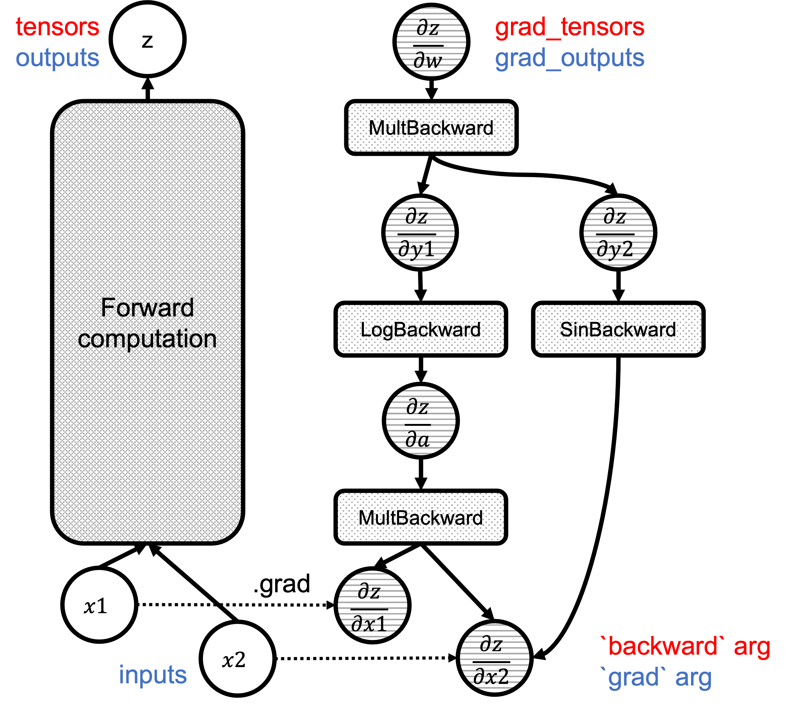
图 1:`backward`/`grad` 参数在图中的对应关系。
深入 Autograd 引擎
概念回顾:节点和边
如我们在 2 中所见,计算图由 Node 和 Edge 对象组成。如果您还没有阅读那篇文章,请务必阅读。
节点
Node 对象在 torch/csrc/autograd/function.h 中定义,它们为关联函数提供 operator() 的重载以及用于图遍历的边列表。请注意,Node 是 autograd 函数继承并重写 apply 方法以执行反向函数的基类。
struct TORCH_API Node : std::enable_shared_from_this<Node> {
 ...
 /// Evaluates the function on the given inputs and returns the result of the
  /// function call.
  variable_list operator()(variable_list&& inputs) {
  ...
  }

protected:
  /// Performs the `Node`'s actual operation.
  virtual variable_list apply(variable_list&& inputs) = 0;
  …
  edge_list next_edges_;
  uint64_t topological_nr_ = 0;
  …
每个节点对象中都有一个名为 topological_nr_ 的属性。此数字用于优化图执行,因为它允许在某些条件下丢弃图分支。拓扑编号是此节点与任何叶节点之间的最长距离,如图 2 所示。其主要特性是,对于有向图中的任何一对节点 x、y,topo_nr(x) < topo_nr(y) 表示没有从 x 到 y 的路径。因此,这可以减少图中需要遍历的路径数量。有关详细信息,请查看 topological_nr 方法注释。
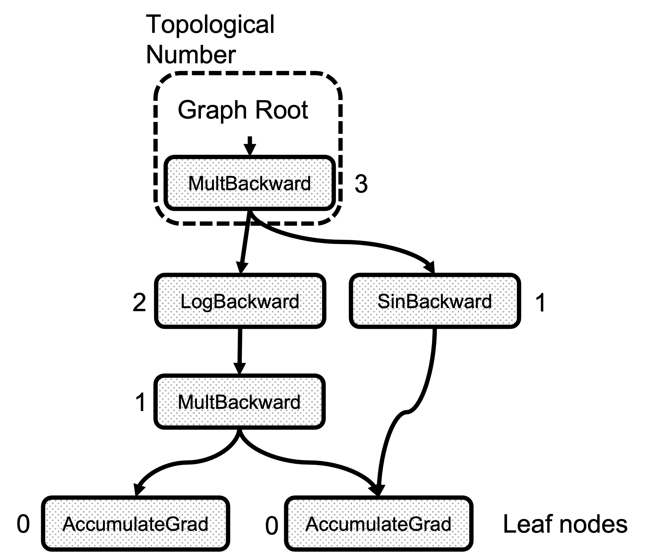
图 2:拓扑编号计算示例
边
Edge 对象将 Nodes 连接在一起,其实现非常简单。
struct Edge {
  ...
  /// The function this `Edge` points to.
  std::shared_ptr<Node> function;
  /// The identifier of a particular input to the function.
  uint32_t input_nr;
};
它只需要一个指向 Node 的函数指针和一个输入编号,该编号是此边指向的前向函数输出的索引。在调用“函数”之前准备梯度集时,我们知道从这条边流出的内容应该累积在“input_nr”参数中。请注意,这里的输入/输出名称是翻转的,这是反向函数的输入。Edge 对象是使用 gradient_edge 函数方法构建的。
 Edge gradient_edge(const Variable& self) {
    if (const auto& gradient = self.grad_fn()) {
      return Edge(gradient, self.output_nr());
    } else {
      return Edge(grad_accumulator(self), 0);
    }
  }
进入 C++ 领域
一旦调用了 torch.autograd.backward(),THPEngine_run_backward 例程就会开始图遍历。以下是函数体的示意图
PyObject *THPEngine_run_backward(PyObject *self, PyObject *args, PyObject *kwargs)
{
  HANDLE_TH_ERRORS
  PyObject *tensors = nullptr;
  PyObject *grad_tensors = nullptr;
  unsigned char keep_graph = 0;
  unsigned char create_graph = 0;
  PyObject *inputs = nullptr;

  // Convert the python arguments to C++ objects
  const char *accepted_kwargs[] = { // NOLINT
      "tensors", "grad_tensors", "keep_graph", "create_graph", "inputs",
      "allow_unreachable", "accumulate_grad", nullptr
  };
  if (!PyArg_ParseTupleAndKeywords(args, kwargs, "OObb|Obb", (char**)accepted_kwargs,
        &tensors, &grad_tensors, &keep_graph, &create_graph, &inputs, &allow_unreachable, &accumulate_grad))

 // Prepare arguments
 for(const auto i : c10::irange(num_tensors)) {
   // Check that the tensors require gradients
  }

  std::vector<Edge> output_edges;
  if (inputs != nullptr) {
     // Prepare outputs
  }

  {
      // Calls the actual autograd engine
    pybind11::gil_scoped_release no_gil;
    outputs = engine.execute(roots, grads, keep_graph, create_graph, accumulate_grad, output_edges);
  }
    // Clean up and finish
}
首先,我们将 PyObject 参数转换为实际的 C++ 对象后,准备输入参数。tensors 列表包含我们开始反向传播的张量。这些张量使用 torch::autograd::impl::gradient_edge 转换为边,并添加到名为 roots 的列表中,图遍历从此处开始。
 edge_list roots;
  roots.reserve(num_tensors);
  variable_list grads;
  grads.reserve(num_tensors);
  for(const auto i : c10::irange(num_tensors)) {
    PyObject *_tensor = PyTuple_GET_ITEM(tensors, i);
       const auto& variable = THPVariable_Unpack(_tensor);
       auto gradient_edge = torch::autograd::impl::gradient_edge(variable);
     roots.push_back(std::move(gradient_edge));

    PyObject *grad = PyTuple_GET_ITEM(grad_tensors, i);
    if (THPVariable_Check(grad)) {
      const Variable& grad_var = THPVariable_Unpack(grad);
      grads.push_back(grad_var);
    }
  }
现在,如果在 backward 中指定了 inputs 参数,或者我们使用了 torch.autograd.grad API,则以下代码会创建一个边列表,用于在计算结束时累积指定张量中的梯度。引擎稍后会使用它来优化执行,因为它不会将梯度添加到所有叶节点,只添加到指定的节点。
  std::vector<Edge> output_edges;
  if (inputs != nullptr) {
    int num_inputs = PyTuple_GET_SIZE(inputs);
    output_edges.reserve(num_inputs);
    for (const auto i : c10::irange(num_inputs)) {
      PyObject *input = PyTuple_GET_ITEM(inputs, i);
      const auto& tensor = THPVariable_Unpack(input);
      const auto output_nr = tensor.output_nr();
      auto grad_fn = tensor.grad_fn();
      if (!grad_fn) {
        grad_fn = torch::autograd::impl::try_get_grad_accumulator(tensor);
      }
      if (accumulate_grad) {
        tensor.retain_grad();
      }
      if (!grad_fn) {
        output_edges.emplace_back(std::make_shared<Identity>(), 0);
      } else {
        output_edges.emplace_back(grad_fn, output_nr);
      }
    }
  }
下一步是实际的图遍历和节点函数执行,最后是清理和返回。
  {
    // Calls the actual autograd engine
    pybind11::gil_scoped_release no_gil;
    auto& engine = python::PythonEngine::get_python_engine();
    outputs = engine.execute(roots, grads, keep_graph, create_graph, accumulate_grad, output_edges);
  }
  // Clean up and finish
}
开始实际执行
engine.execute 位于 torch/csrc/autograd/engine.cpp
这里有两个不同的步骤
分析图以查找函数之间的依赖关系 创建遍历图的工作线程
用于执行的数据结构
GraphTask
所有执行元数据都由 GraphTask 类在 torch/csrc/autograd/engine.h 中管理
struct GraphTask: std::enable_shared_from_this<GraphTask> {
  std::atomic<uint64_t> outstanding_tasks_{0};
  //  …
  std::unordered_map<Node*, InputBuffer> not_ready_;
  std::unordered_map<Node*, int> dependencies_;

  struct ExecInfo {
     // …
  };
  std::unordered_map<Node*, ExecInfo> exec_info_;
  std::vector<Variable> captured_vars_;
  // …
  std::shared_ptr<ReadyQueue> cpu_ready_queue_;
};
在这里,我们看到了一系列用于维护执行状态的变量。outstanding_tasks_ 跟踪反向传播完成所需执行的任务数量。not_ready_ 存储尚未准备好执行的 Nodes 的输入参数。dependencies_ 跟踪 Node 拥有的前驱数量。当计数达到 0 时,Node 即可执行;它被放入一个就绪队列中,稍后检索并执行。
exec_info_ 和关联的 ExecInfo 结构仅在指定了 inputs 参数或调用 autograd.grad() 时使用。它们允许过滤图中不需要的路径,因为梯度仅针对 inputs 列表中的变量计算。
如果我们使用 torch.autograd.grad() API 而不是 torch.autograd.backward(),captured_vars_ 是图执行结果临时存储的地方,因为 grad() 返回梯度作为张量,而不是仅仅填充输入的 .grad 字段。
NodeTask
NodeTask 结构体是一个基本类,它包含一个指向要执行的节点的 fn_ 指针和一个 inputs_ 缓冲区,用于存储此函数的输入参数。请注意,反向传播执行的函数是 derivatives.yaml 文件中指定的导数,或者是第二篇博客文章中描述的使用自定义函数时用户提供的反向函数。
inputs_ 缓冲区也是聚合先前执行函数的输出梯度的地方,它被定义为 std::vector 容器,具有在给定位置累积值的功能。
struct NodeTask {
  std::weak_ptr<GraphTask> base_;
  std::shared_ptr<Node> fn_;
  // This buffer serves as an implicit "addition" node for all of the
  // gradients flowing here.  Once all the dependencies are finished, we
  // use the contents of this buffer to run the function.
  InputBuffer inputs_;
};
GraphRoot
GraphRoot 是一个特殊函数,用于在一个地方保存多个输入变量。代码非常简单,因为它只充当变量的容器。
struct TORCH_API GraphRoot : public Node {
  GraphRoot(edge_list functions, variable_list inputs)
      : Node(std::move(functions)),
      outputs(std::move(inputs)) {
    for (const auto& t : outputs) {
      add_input_metadata(t);
    }
  }

  variable_list apply(variable_list&& inputs) override {
    return outputs;
  }
AccumulateGrad
当 Variable 对象没有 grad_fn 时,此函数在 gradient_edge 中的图创建期间设置。也就是说,它是一个叶节点。
    if (const auto& gradient = self.grad_fn()) {
      // …
    } else {
      return Edge(grad_accumulator(self), 0);
    }
函数体在 torch/csrc/autograd/functions/accumulate_grad.cpp 中定义,它主要将输入梯度累积到对象的 .grad 属性中。
auto AccumulateGrad::apply(variable_list&& grads) -> variable_list {
  check_input_variables("AccumulateGrad", grads, 1, 0);
  …

  at::Tensor new_grad = callHooks(variable, std::move(grads[0]));
  std::lock_guard<std::mutex> lock(mutex_);

  at::Tensor& grad = variable.mutable_grad();
  accumulateGrad(
      variable,
      grad,
      new_grad,
      1 + !post_hooks().empty() /* num_expected_refs */,
      [&grad](at::Tensor&& grad_update) { grad = std::move(grad_update); });
  return variable_list();
}
}} // namespace torch::autograd
accumulateGrad 对张量格式进行多次检查,并最终执行 variable_grad += new_grad; 累积。
准备图执行
现在,让我们来阅读 Engine::execute。除了参数一致性检查之外,要做的第一件事是创建我们上面描述的实际 GraphTask 对象。此对象保存了图执行的所有元数据。
auto Engine::execute(const edge_list& roots,
                     const variable_list& inputs,
                     bool keep_graph,
                     bool create_graph,
                     bool accumulate_grad,
                     const edge_list& outputs) -> variable_list {

  validate_outputs(roots, const_cast<variable_list&>(inputs), [](const std::string& msg) {
    return msg;
  });

  // Checks

  auto graph_task = std::make_shared<GraphTask>(
      /* keep_graph */ keep_graph,
      /* create_graph */ create_graph,
      /* depth */ not_reentrant_backward_call ? 0 : total_depth + 1,
      /* cpu_ready_queue */ local_ready_queue);

  // If we receive a single root, skip creating extra root node
  // …
  // Prepare graph by computing dependencies
  // …
  // Queue the root
  // …
  // launch execution
  // …
}
创建 GraphTask 后,如果我们只有一个根节点,则使用其关联函数。如果存在多个根节点,则创建如前所述的特殊 GraphRoot 对象。
  bool skip_dummy_node = roots.size() == 1;
  auto graph_root = skip_dummy_node ?
    roots.at(0).function :
    std::make_shared<GraphRoot>(roots, inputs);
下一步是填充 GraphTask 对象中的 dependencies_ 映射,因为引擎必须知道何时可以执行任务。这里的 outputs 是传递给 Python 中 torch.autograd.backward() 调用的 inputs 参数。但是这里我们反转了名称,因为相对于前向传播输入的梯度现在是反向传播的输出。从现在开始,没有前向/反向的概念,只有图遍历和执行。
  auto min_topo_nr = compute_min_topological_nr(outputs);
  // Now compute the dependencies for all executable functions
  compute_dependencies(graph_root.get(), *graph_task, min_topo_nr);

  if (!outputs.empty()) {
    graph_task->init_to_execute(*graph_root, outputs, accumulate_grad, min_topo_nr);
  }
在这里,我们预处理图以执行节点。首先,调用 compute_min_topological_nr 来获取 outputs 中指定的张量的最小拓扑编号(如果没有向 .backward 或 .grad 提供 inputs 关键字参数,则为 0)。此计算会修剪图中导致我们不需要/不计算梯度的输入变量的路径。
其次是 compute_dependencies 调用。此函数是一个非常简单的图遍历,从根 Node 开始,对于 node.next_edges() 中的每个边,它会递增 dependencies_ 中的计数器。图 3 显示了示例图中依赖关系计算的结果。请注意,任何节点的依赖关系数量只是到达它的边数。
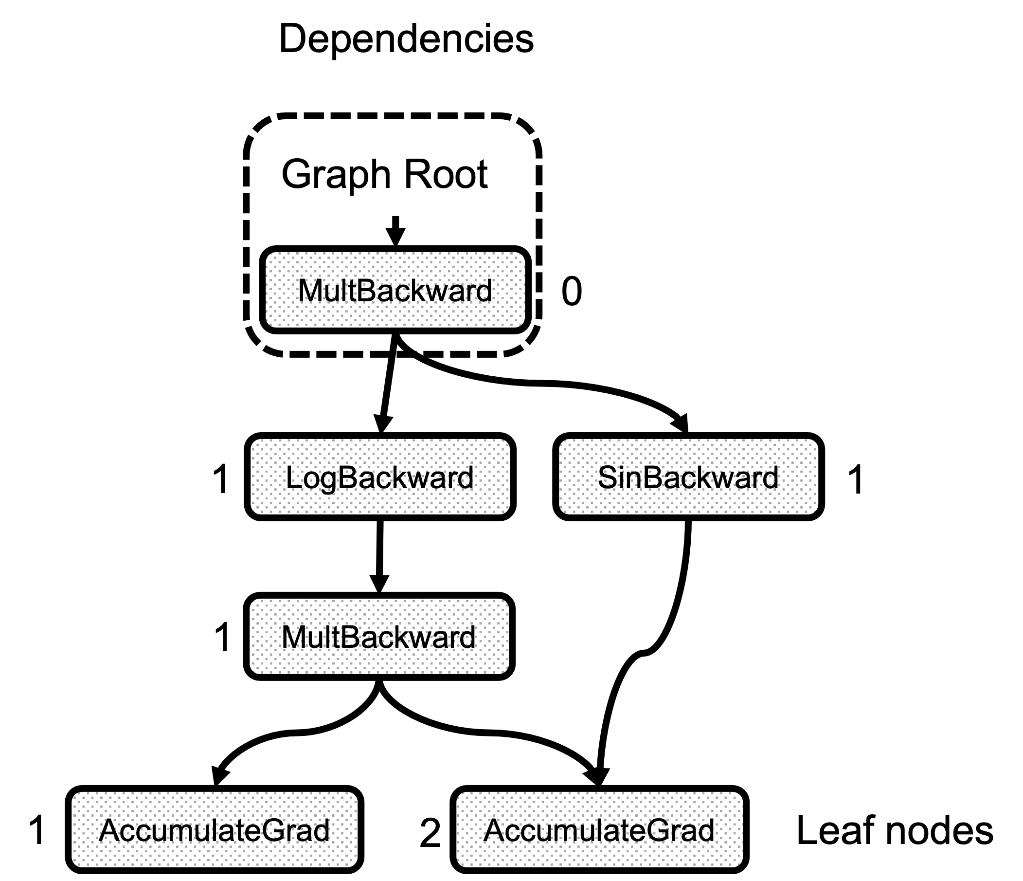
图 3:每个节点的依赖关系数量
最后,调用 init_to_execute,这会在 Python backward 调用中指定 inputs 的情况下填充 GraphTask::exec_info_ 映射。它再次遍历图,从根开始,并在 exec_info_ 映射中记录仅计算给定 inputs 梯度所需的中间节点。
  // Queue the root
  if (skip_dummy_node) {
    InputBuffer input_buffer(roots.at(0).function->num_inputs());
    auto input = inputs.at(0);


    input_buffer.add(roots.at(0).input_nr,
                      std::move(input),
                      input_stream,
                      opt_next_stream);

    execute_with_graph_task(graph_task, graph_root, std::move(input_buffer));
  } else {
    execute_with_graph_task(graph_task, graph_root, InputBuffer(variable_list()));
  }
  // Avoid a refcount bump for the Future, since we check for refcount in
  // DistEngine (see TORCH_INTERNAL_ASSERT(futureGrads.use_count() == 1)
  // in dist_engine.cpp).
  auto& fut = graph_task->future_result_;
  fut->wait();
  return fut->value().toTensorVector();
}
现在,我们准备通过创建 InputBuffer 来开始实际执行。如果我们只有一个根变量,我们首先将 inputs 张量的值(这是传递给 python backward 的 gradients)复制到 input_buffer 的位置 0。这是一个小的优化,避免了无缘无故地运行 RootNode。此外,如果图的其余部分不在 CPU 上,我们直接在该工作线程上开始,而 RootNode 始终放置在 CPU 就绪队列中。工作线程和就绪队列的详细信息将在下面的部分中解释。
另一方面,如果我们有多个根,GraphRoot 对象也持有输入,因此只需向其传递一个空的 InputBuffer。
图遍历和节点执行
设备、线程和队列
在深入实际执行之前,我们需要了解引擎的结构。
首先,引擎是多线程的,每个设备一个线程。例如,调用线程与 CPU 相关联,而为系统中可用的每个 GPU 或其他设备创建并关联额外的线程。每个线程都使用 worker_device 变量中的线程局部存储跟踪其设备。此外,线程有一个任务队列要执行,也位于线程局部存储中,即 local_ready_queue。这是工作线程在此线程中排队以在稍后解释的 thread_main 函数中执行的地方。您会想知道如何决定执行任务的设备。InputBuffer 类有一个 device() 函数,它返回其所有张量的第一个非 CPU 设备。此函数与 Engine::ready_queue 一起使用来选择要排队任务的队列。
auto Engine::ready_queue(std::shared_ptr<ReadyQueue> cpu_ready_queue, at::Device device) -> std::shared_ptr<ReadyQueue>{
  if (device.type() == at::kCPU || device.type() == at::DeviceType::Meta) {
    return cpu_ready_queue;
  } else {
    // See Note [Allocating GPUs to autograd threads]
    return device_ready_queues_.at(device.index());
  }
}
ReadyQueue 对象在 torch/csrc/autograd/engine.h 中定义,它是一个简单的 std::priority_queue 包装器,允许线程在为空时 等待任务。ReadyQueue 的一个有趣属性是它会增加用于确定执行是否完成的 GraphTask::outstanding_tasks_ 值。
auto ReadyQueue::push(NodeTask item, bool incrementOutstandingTasks) -> void {
  {
    std::lock_guard<std::mutex> lock(mutex_);
    if (incrementOutstandingTasks) {
      std::shared_ptr<GraphTask> graph_task = item.base_.lock();
      ++graph_task->outstanding_tasks_;
    }
    heap_.push(std::move(item));
  }
  not_empty_.notify_one();
}

auto ReadyQueue::pop() -> NodeTask {
  std::unique_lock<std::mutex> lock(mutex_);
  not_empty_.wait(lock, [this]{ return !heap_.empty(); });
  auto task = std::move(const_cast<NodeTask&>(heap_.top())); heap_.pop();
  return task;
}
可重入反向传播
当反向传播中的一个任务再次调用 backward 时,就会发生可重入反向传播。这不是一个非常常见的情况,但它可以通过避免保存中间结果来减少内存使用。欲了解更多信息,请查看这篇 PyTorch 论坛帖子。
class ReentrantBackward(torch.autograd.Function):
    @staticmethod
    def forward(ctx, input):
        return input.sum()

    @staticmethod
    def backward(ctx, input):
        # Let's compute the backward by using autograd
        input = input.detach().requires_grad_()
        with torch.enable_grad():
            out = input.sum()
        out.backward()  # REENTRANT CALL!!
        return out.detach()
这里,我们在用户自定义的 autograd 函数中调用了 backward()。这种情况可能导致死锁,因为第一个 backward 需要等待第二个 backward 完成。但是,一些内部实现细节可能会阻止第二个 backward 完成,这将在专门的小节中解释。
线程初始化
execute_with_graph_task 负责初始化负责计算的线程并将 root 节点放入生成它的设备的队列中。
c10::intrusive_ptr<at::ivalue::Future> Engine::execute_with_graph_task(
    const std::shared_ptr<GraphTask>& graph_task,
    std::shared_ptr<Node> graph_root,
    InputBuffer&& input_buffer) {

  initialize_device_threads_pool();
  // Lock mutex for GraphTask.
  std::unique_lock<std::mutex> lock(graph_task->mutex_);

  auto queue = ready_queue(graph_task->cpu_ready_queue_, input_buffer.device());

  if (worker_device == NO_DEVICE) {
    set_device(CPU_DEVICE);
    graph_task->owner_ = worker_device;
    queue->push(NodeTask(graph_task, std::move(graph_root), std::move(input_buffer)));
    lock.unlock();
    thread_main(graph_task);
    worker_device = NO_DEVICE;
  } else {
     // This deals with reentrant backwards, we will see it later.
  }
  return graph_task->future_result_;
}
首先,此函数通过调用 initialize_device_threads_pool() 初始化多个线程(每个设备一个),在此过程中会发生以下几件事:为每个设备创建一个 ReadyQueue。为每个非 CPU 设备创建一个线程。设置一个线程局部 worker_device 变量以跟踪与线程关联的当前设备。调用 thread_main 函数,并且线程等待任务被放入其队列中。
然后,它使用 ready_queue 函数根据持有 input_buffer 中存在的张量的设备检索队列以放置根节点。现在,主线程(也执行 Python 解释器的线程)的 worker_device 设置为 NO_DEVICE,它负责执行所有张量都在 CPU 中的函数。如果 worker_device 设置为任何其他值,则图执行已经开始,并且在运行中的 Node 内部调用了 .backward(),从而创建了可重入的反向调用。这将在后面解释。目前,主线程将任务放入队列并调用 thread_main。
奇迹发生的地方
路漫漫,但我们终于可以遍历图并执行节点了。每个派生线程和主线程都调用 thread_main。
auto Engine::thread_main(const std::shared_ptr<GraphTask>& graph_task) -> void {

  while (graph_task == nullptr || !graph_task->future_result_->completed()) {
    std::shared_ptr<GraphTask> local_graph_task;
    {
      NodeTask task = local_ready_queue->pop();

      if (task.isShutdownTask_) {
        break;
      }

      if (!(local_graph_task = task.base_.lock())) {
        // GraphTask for function is no longer valid, skipping further
        // execution.
        continue;
      }

      if (task.fn_ && !local_graph_task->has_error_.load()) {
        at::ThreadLocalStateGuard tls_guard(local_graph_task->thread_locals_);

        try {
          GraphTaskGuard guard(local_graph_task);
          NodeGuard ndguard(task.fn_);
          {
            evaluate_function(
                local_graph_task,
                task.fn_.get(),
                task.inputs_,
                local_graph_task->cpu_ready_queue_);
          }
        } catch (std::exception& e) {
          thread_on_exception(local_graph_task, task.fn_, e);
        }
      }
    }

    // Decrement the outstanding tasks.
    --local_graph_task->outstanding_tasks_;

    // Check if we've completed execution.
    if (local_graph_task->completed()) {
      local_graph_task->mark_as_completed_and_run_post_processing();
      auto base_owner = local_graph_task->owner_;
      if (worker_device != base_owner) {
        std::atomic_thread_fence(std::memory_order_release);
        ready_queue_by_index(local_graph_task->cpu_ready_queue_, base_owner)
            ->push(NodeTask(local_graph_task, nullptr, InputBuffer(0)));
      }
    }
  }
}
这里的代码很简单,给定分配给每个线程的线程局部存储中的 local_ready_queue。线程循环直到图中没有任务可执行。请注意,对于设备关联线程,传递的 graph_task 参数是 nullptr,它们在 local_ready_queue->pop() 中阻塞,直到任务被推入它们的队列。经过一些一致性检查(任务类型是关闭,或者图仍然有效)。我们进入 evaluate_function 中的实际函数调用。
        try {
          GraphTaskGuard guard(local_graph_task);
          NodeGuard ndguard(task.fn_);
          {
            evaluate_function(
                local_graph_task,
                task.fn_.get(),
                task.inputs_,
                local_graph_task->cpu_ready_queue_);
          }
        } catch (std::exception& e) {
          thread_on_exception(local_graph_task, task.fn_, e);
        }
      }
调用 evaluate_function 后,我们通过查看 outstanding_tasks_ 数量来检查 graph_task 执行是否完成。当任务被推入队列时,此数量会增加,当任务执行完毕后,在 local_graph_task->completed() 中减少。当执行完成时,我们返回结果,如果调用的是 torch.autograd.grad() 而不是 torch.autograd.backward(),结果将存储在 captured_vars_ 中,因为此函数返回张量而不是将它们存储在输入的 .grad 属性中。最后,如果主线程正在等待,我们通过发送一个虚拟任务来唤醒它。
   // Decrement the outstanding tasks.
    --local_graph_task->outstanding_tasks_;

    // Check if we've completed execution.
    if (local_graph_task->completed()) {
      local_graph_task->mark_as_completed_and_run_post_processing();
      auto base_owner = local_graph_task->owner_;
      if (worker_device != base_owner) {
        std::atomic_thread_fence(std::memory_order_release);
        ready_queue_by_index(local_graph_task->cpu_ready_queue_, base_owner)
            ->push(NodeTask(local_graph_task, nullptr, InputBuffer(0)));
      }
    }
调用函数并解锁新任务
evaluate_function 有三个目的
运行函数。将其结果累积到下一个节点的 InputBuffers 中。减少下一个节点的依赖计数器,并将达到 0 的任务入队以执行。
void Engine::evaluate_function(
    std::shared_ptr<GraphTask>& graph_task,
    Node* func,
    InputBuffer& inputs,
    const std::shared_ptr<ReadyQueue>& cpu_ready_queue) {

  // If exec_info_ is not empty, we have to instrument the execution
  auto& exec_info_ = graph_task->exec_info_;
  if (!exec_info_.empty()) {
    // Checks if the function needs to be executed
    if (!fn_info.needed_) {
      // Skip execution if we don't need to execute the function.
      return;
    }
  }

  auto outputs = call_function(graph_task, func, inputs);

  auto& fn = *func;
  if (!graph_task->keep_graph_) {
    fn.release_variables();
  }
最初,我们检查 GraphTask 结构的 exec_info_ 映射,以确定当前节点是否需要执行。请记住,如果此映射为空,则所有节点都将执行,因为我们正在计算前向传播所有输入的梯度。
经过此检查后,通过运行 call_function 来执行该函数。其实现非常直接,并调用实际的导数函数(如果有的话)和注册的钩子。
  int num_outputs = outputs.size();
  if (num_outputs == 0) {
    // Records leaf stream (if applicable)
    return;
  }

  if (AnomalyMode::is_enabled()) {
    // check for nan values in result
  }
接下来,在 call_function 完成后,我们检查函数的输出。如果输出数量为 0,则没有要执行的后续节点,因此我们可以安全地返回。这是与叶节点关联的 AccumulateGrad 节点的情况。
此外,如果需要,还在此处检查梯度中的 NaN 值。
  std::lock_guard<std::mutex> lock(graph_task->mutex_);
  for (const auto i : c10::irange(num_outputs)) {
    auto& output = outputs[i];
    const auto& next = fn.next_edge(i);

    if (!next.is_valid()) continue;
我们现在执行了一个 grad_fn,它为每个关联的前向传播函数输入返回一个梯度。正如我们在上一篇博客文章中看到的,我们为每个这些输入张量都有一个 Edge 对象,以及前向传播中生成它们的函数的 grad_fn。本质上,反向传播中节点的 Output[0] 对应于前向传播关联函数的第一个参数。图 4 显示了反向函数的输出与前向函数输入之间的关系。请注意,grad_fn C 的输出是 z 相对于 Function C 输入的梯度。
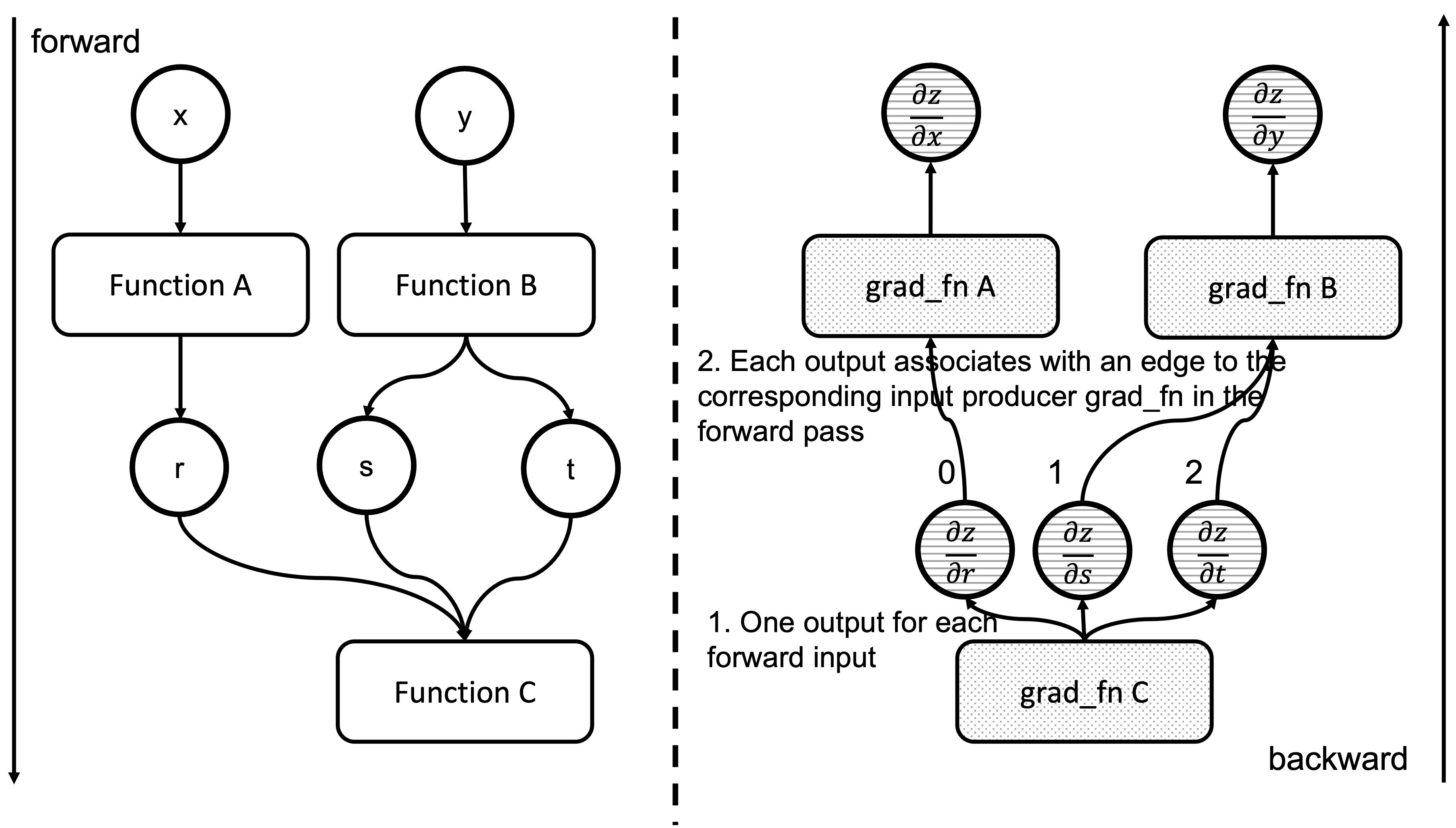
图 4:前向和反向函数输入和输出之间的对应关系
现在我们遍历这些边,并检查关联的函数是否已准备好执行。
 // Check if the next function is ready to be computed
    bool is_ready = false;
    auto& dependencies = graph_task->dependencies_;
    auto it = dependencies.find(next.function.get());

    if (it == dependencies.end()) {
      auto name = next.function->name();
      throw std::runtime_error(std::string("dependency not found for ") + name);
    } else if (--it->second == 0) {
      dependencies.erase(it);
      is_ready = true;
    }

    auto& not_ready = graph_task->not_ready_;
    auto not_ready_it = not_ready.find(next.function.get());
为此,我们检查 graph_task->dependencies_ 映射。我们递减计数器,如果它达到 0,则将边指向的函数标记为准备好执行。接下来,我们准备由下一个边指示的任务的输入缓冲区。
    if (not_ready_it == not_ready.end()) {
      if (!exec_info_.empty()) {
        // Skip functions that aren't supposed to be executed
      }

      // Creates an InputBuffer and moves the output to the corresponding input position
      InputBuffer input_buffer(next.function->num_inputs());
      input_buffer.add(next.input_nr,
                       std::move(output),
                       opt_parent_stream,
                       opt_next_stream);

      if (is_ready) {
        auto queue = ready_queue(cpu_ready_queue, input_buffer.device());
        queue->push(
            NodeTask(graph_task, next.function, std::move(input_buffer)));
      } else {
        not_ready.emplace(next.function.get(), std::move(input_buffer));
      }
在这里,我们在 graph_task->not_ready_ 映射中查找任务。如果它不存在,我们创建一个新的 InputBuffer 对象,并将当前输出设置为与边关联的缓冲区中的 input_nr 位置。如果任务已准备好执行,我们将其排入适当的设备 ready_queue 并完成执行。但是,如果任务未准备好且我们之前已经看到过它,则它存在于 not_ready_map_ 中。
    } else {
      // The function already has a buffer
      auto &input_buffer = not_ready_it->second;
      // Accumulates into buffer
      input_buffer.add(next.input_nr,
                       std::move(output),
                       opt_parent_stream,
                       opt_next_stream);
      if (is_ready) {
        auto queue = ready_queue(cpu_ready_queue, input_buffer.device());
        queue->push(NodeTask(graph_task, next.function, std::move(input_buffer)));
        not_ready.erase(not_ready_it);
      }
    }
  }
}
在这种情况下,我们将输出累积到现有的 input_buffer 中,而不是创建一个新的。一旦所有任务都处理完毕,工作线程退出循环并完成。所有这些过程都在图 5 的动画中总结。我们看到一个线程如何查看就绪队列中的任务并减少下一个节点的依赖关系,从而解锁它们以执行。
图 5:计算图执行动画
可重入反向传播流程
正如我们上面看到的,可重入反向传播问题是指当前执行的函数再次调用 backward。发生这种情况时,运行此函数的线程会一直向下到 execute_with_graph_task,与非可重入情况一样,但这里情况有所不同。
c10::intrusive_ptr<at::ivalue::Future> Engine::execute_with_graph_task(
    const std::shared_ptr<GraphTask>& graph_task,
    std::shared_ptr<Node> graph_root,
    InputBuffer&& input_buffer) {

  initialize_device_threads_pool();
  // Lock mutex for GraphTask.
  std::unique_lock<std::mutex> lock(graph_task->mutex_);

  auto queue = ready_queue(graph_task->cpu_ready_queue_, input_buffer.device());

  if (worker_device == NO_DEVICE) {
    //Regular case
  } else {
    // If worker_device is any devices (i.e. CPU, CUDA): this is a re-entrant
    //    backward call from that device.
    graph_task->owner_ = worker_device;

    // Now that all the non-thread safe fields of the graph_task have been populated,
    // we can enqueue it.
    queue->push(NodeTask(graph_task, std::move(graph_root), std::move(input_buffer)));

    if (current_depth >= max_recursion_depth_) {
      // If reached the max depth, switch to a different thread
      add_thread_pool_task(graph_task);
    } else {
      ++total_depth;
      ++current_depth;
      lock.unlock();
      thread_main(graph_task);
      --current_depth;
      --total_depth;
    }
  }
  return graph_task->future_result_;
}
在这里,execute_with_graph_task 将其检测为可重入调用,然后查找当前嵌套调用的数量。如果超出限制,我们创建一个新线程来处理此图的执行,否则,我们正常执行此可重入调用。最初设置嵌套调用限制是为了避免因可重入调用创建非常大的调用堆栈而导致的堆栈溢出。然而,当添加 sanitizer 测试时,由于线程在给定时刻可以持有的最大锁量,该数字进一步减小。这可以在 torch/csrc/autograd/engine.h 中看到。
当超过此最大深度时,会使用 add_thread_pool_task 函数创建一个新线程。
void Engine::add_thread_pool_task(const std::weak_ptr<GraphTask>& graph_task) {
  std::unique_lock<std::mutex> lck(thread_pool_shared_->mutex_);
  // if we have pending graph_task objects to be processed, create a worker.
   bool create_thread = (thread_pool_shared_->num_workers_ <= thread_pool_shared_->graphtasks_queue_.size());
  thread_pool_shared_->graphtasks_queue_.push(graph_task);


  lck.unlock();
  if (create_thread) {
    std::thread t(&Engine::reentrant_thread_init, this);
    t.detach();
  }

  thread_pool_shared_->work_.notify_one();
}
在深入探讨之前,让我们看一下 Engine 中的 thread_pool_shared_ 对象,它管理与可重入反向调用关联的线程的所有信息。
  struct ThreadPoolShared {
    unsigned int num_workers_;
    std::condition_variable work_;
    std::mutex mutex_;
    std::queue<std::weak_ptr<GraphTask>> graphtasks_queue_;

    // NOLINTNEXTLINE(cppcoreguidelines-pro-type-member-init)
    ThreadPoolShared() : num_workers_(0) {}
 };
ThreadPoolShared 是一个简单的容器,包含一个 GraphTask 对象队列,带有同步机制和当前工作线程数量。
现在很容易理解 add_thread_pool_task 如何在 graph_task 对象入队且没有足够的工作线程来处理它们时创建线程。
add_thread_pool_task 通过执行 reentrant_thread_init 来初始化线程。
void Engine::reentrant_thread_init() {
  at::init_num_threads();
  auto tp_shared = thread_pool_shared_;
  while(true) {
    std::unique_lock<std::mutex> lk(tp_shared->mutex_);
    ++thread_pool_shared_->num_workers_;
    tp_shared->work_.wait(lk, [&tp_shared]{ return !tp_shared->graphtasks_queue_.empty();});
    --thread_pool_shared_->num_workers_;
    auto task = tp_shared->graphtasks_queue_.front();
    tp_shared->graphtasks_queue_.pop();
    lk.unlock();
    std::shared_ptr<GraphTask> graph_task;
    if (!(graph_task = task.lock())) {
      continue;
    }
    set_device(graph_task->owner_);
    // set the local_ready_queue to the ready queue on the graph_task->owner_ device
    local_ready_queue = ready_queue_by_index(graph_task->cpu_ready_queue_, graph_task->owner_);
    total_depth = graph_task->reentrant_depth_;
    thread_main(graph_task);
  }
}
代码很简单。新创建的线程在 thread_pool_shared->graphtasks_queue_ 上等待可重入反向图可用并执行它们。请注意,此线程通过访问在 execute_with_graph_task 函数中设置的 graph_task->owner_ 字段,使用与启动此调用的线程设备关联的任务就绪队列。
错误处理
每当其中一个工作线程发生错误时,它都会传播到调用 backward 的线程。
为此,thread_main 中有一个 try/catch 块,用于捕获 Node 函数调用中的任何异常,并将其设置为关联的 GraphTask 对象。
       try {
          …
          GraphTaskGuard guard(local_graph_task);
          NodeGuard ndguard(task.fn_);
          {
            evaluate_function(
               …
          }
        } catch (std::exception& e) {
          thread_on_exception(local_graph_task, task.fn_, e);
        }
      }
    }
thread_on_exception 及其调用的函数最终会在 local_graph_task 对象中设置异常。
void Engine::thread_on_exception(
    std::shared_ptr<GraphTask> graph_task,
    const std::shared_ptr<Node>& fn,
    std::exception& e) {
  graph_task->set_exception(std::current_exception(), fn);
}

void GraphTask::set_exception_without_signal(const std::shared_ptr<Node>& fn) {
  if (!has_error_.exchange(true)) {
    if (AnomalyMode::is_enabled() && fn) {
      fn->metadata()->print_stack(fn->name());
    }
  }
}

void GraphTask::set_exception(
    std::exception_ptr eptr,
    const std::shared_ptr<Node>& fn) {
  set_exception_without_signal(fn);
  if (!future_completed_.exchange(true)) {
    // NOLINTNEXTLINE(performance-move-const-arg)
    future_result_->setError(std::move(eptr));
  }
}
在 set_exception 中,它将 has_error_ 标志设置为 true,并调用 setError 函数 future_result_ 对象。当访问 future_result_->value() 时,这将导致错误在调用线程中重新抛出。
 IValue value() {
    std::unique_lock<std::mutex> lock(mutex_);
    AT_ASSERT(completed());
    if (eptr_) {
      std::rethrow_exception(eptr_);
    }
    return value_;
  }
结语
这是本系列的最后一篇文章,涵盖了 PyTorch 如何进行自动微分。我们希望您喜欢阅读它,并且现在您已经足够熟悉 PyTorch 内部结构,可以开始为 PyTorch 开发做出贡献了!