可视化实用工具

注意

在 collab 上尝试或 转到末尾 下载完整的示例代码。

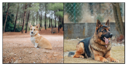
此示例说明了 torchvision 提供的一些用于可视化图像、边界框、分割掩模和关键点的实用工具。

import torch
import numpy as np
import matplotlib.pyplot as plt

import torchvision.transforms.functional as F


plt.rcParams["savefig.bbox"] = 'tight'


def show(imgs):
    if not isinstance(imgs, list):
        imgs = [imgs]
    fig, axs = plt.subplots(ncols=len(imgs), squeeze=False)
    for i, img in enumerate(imgs):
        img = img.detach()
        img = F.to_pil_image(img)
        axs[0, i].imshow(np.asarray(img))
        axs[0, i].set(xticklabels=[], yticklabels=[], xticks=[], yticks=[])

可视化图像网格

可以使用 make_grid() 函数创建一个表示网格中多个图像的张量。此实用工具要求输入一个数据类型为 uint8 的单个图像。

from torchvision.utils import make_grid
from torchvision.io import read_image
from pathlib import Path

dog1_int = read_image(str(Path('../assets') / 'dog1.jpg'))
dog2_int = read_image(str(Path('../assets') / 'dog2.jpg'))
dog_list = [dog1_int, dog2_int]

grid = make_grid(dog_list)
show(grid)

可视化边界框

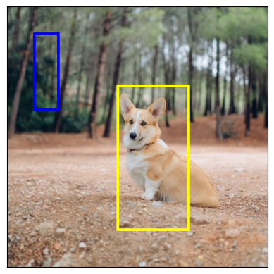
我们可以使用 draw_bounding_boxes() 在图像上绘制框。我们可以设置颜色、标签、宽度以及字体和字体大小。框的格式为 (xmin, ymin, xmax, ymax)。

from torchvision.utils import draw_bounding_boxes


boxes = torch.tensor([[50, 50, 100, 200], [210, 150, 350, 430]], dtype=torch.float)
colors = ["blue", "yellow"]
result = draw_bounding_boxes(dog1_int, boxes, colors=colors, width=5)
show(result)

自然地，我们还可以绘制 torchvision 检测模型生成的边界框。以下是从 fasterrcnn_resnet50_fpn() 模型加载的 Faster R-CNN 模型的演示。有关此类模型输出的更多详细信息，请参阅 实例分割模型。

from torchvision.models.detection import fasterrcnn_resnet50_fpn, FasterRCNN_ResNet50_FPN_Weights


weights = FasterRCNN_ResNet50_FPN_Weights.DEFAULT
transforms = weights.transforms()

images = [transforms(d) for d in dog_list]

model = fasterrcnn_resnet50_fpn(weights=weights, progress=False)
model = model.eval()

outputs = model(images)
print(outputs)

[{'boxes': tensor([[215.9767, 171.1661, 402.0078, 378.7391],
        [344.6341, 172.6735, 357.6114, 220.1435],
        [153.1306, 185.5567, 172.9223, 254.7014]], grad_fn=<StackBackward0>), 'labels': tensor([18,  1,  1]), 'scores': tensor([0.9989, 0.0701, 0.0611], grad_fn=<IndexBackward0>)}, {'boxes': tensor([[ 23.5964, 132.4331, 449.9359, 493.0222],
        [225.8182, 124.6292, 467.2861, 492.2621],
        [ 18.5248, 135.4171, 420.9786, 479.2225]], grad_fn=<StackBackward0>), 'labels': tensor([18, 18, 17]), 'scores': tensor([0.9980, 0.0879, 0.0671], grad_fn=<IndexBackward0>)}]

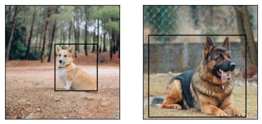
让我们绘制模型检测到的框。我们只绘制得分高于给定阈值的框。

score_threshold = .8
dogs_with_boxes = [
    draw_bounding_boxes(dog_int, boxes=output['boxes'][output['scores'] > score_threshold], width=4)
    for dog_int, output in zip(dog_list, outputs)
]
show(dogs_with_boxes)

可视化分割蒙版

函数 draw_segmentation_masks() 可用于在图像上绘制分割蒙版。语义分割和实例分割模型具有不同的输出，因此我们将分别处理每个模型。

语义分割模型

我们将了解如何将其与 torchvision 的 FCN Resnet-50 配合使用，该模型使用 fcn_resnet50() 加载。让我们首先了解模型的输出。

from torchvision.models.segmentation import fcn_resnet50, FCN_ResNet50_Weights

weights = FCN_ResNet50_Weights.DEFAULT
transforms = weights.transforms(resize_size=None)

model = fcn_resnet50(weights=weights, progress=False)
model = model.eval()

batch = torch.stack([transforms(d) for d in dog_list])
output = model(batch)['out']
print(output.shape, output.min().item(), output.max().item())

Downloading: "https://download.pytorch.org/models/fcn_resnet50_coco-1167a1af.pth" to /root/.cache/torch/hub/checkpoints/fcn_resnet50_coco-1167a1af.pth
torch.Size([2, 21, 500, 500]) -7.089669704437256 14.858257293701172

如上所述，分割模型的输出是形状为 (batch_size, num_classes, H, W) 的张量。每个值都是非归一化分数，我们可以使用 softmax 将它们归一化为 [0, 1]。在 softmax 之后，我们可以将每个值解释为一个概率，表示给定像素属于给定类的可能性。

让我们绘制针对狗类和船类检测到的蒙版

sem_class_to_idx = {cls: idx for (idx, cls) in enumerate(weights.meta["categories"])}

normalized_masks = torch.nn.functional.softmax(output, dim=1)

dog_and_boat_masks = [
    normalized_masks[img_idx, sem_class_to_idx[cls]]
    for img_idx in range(len(dog_list))
    for cls in ('dog', 'boat')
]

show(dog_and_boat_masks)

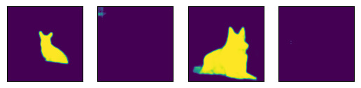
正如预期的那样，该模型对狗类很有信心，但对船类则不太有信心。

可以使用 draw_segmentation_masks() 函数在原始图像上绘制这些蒙版。此函数期望蒙版是布尔蒙版，但我们上面的蒙版包含 [0, 1] 中的概率。为了获得布尔蒙版，我们可以执行以下操作

class_dim = 1
boolean_dog_masks = (normalized_masks.argmax(class_dim) == sem_class_to_idx['dog'])
print(f"shape = {boolean_dog_masks.shape}, dtype = {boolean_dog_masks.dtype}")
show([m.float() for m in boolean_dog_masks])

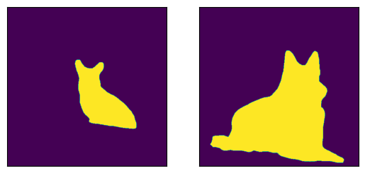
shape = torch.Size([2, 500, 500]), dtype = torch.bool

我们在其中定义 boolean_dog_masks 的上述行有点晦涩，但你可以将它理解为以下查询：“对于哪些像素，“狗”是最可能的类？”

注意

虽然我们在此处使用 normalized_masks，但我们直接使用模型的非归一化分数也会获得相同的结果（因为 softmax 操作保留了顺序）。

现在我们有了布尔蒙版，我们可以将它们与 draw_segmentation_masks() 一起使用，将它们绘制在原始图像之上

from torchvision.utils import draw_segmentation_masks

dogs_with_masks = [
    draw_segmentation_masks(img, masks=mask, alpha=0.7)
    for img, mask in zip(dog_list, boolean_dog_masks)
]
show(dogs_with_masks)

我们可以为每张图像绘制多个蒙版！请记住，该模型返回的蒙版与类一样多。让我们提出与上面相同的问题，但这次针对所有类，而不仅仅是狗类：“对于每个像素和每个类 C，类 C 是否是最可能的类？”

这一问题有点复杂，因此我们首先展示如何使用单个图像来解决它，然后我们将它推广到批处理

num_classes = normalized_masks.shape[1]
dog1_masks = normalized_masks[0]
class_dim = 0
dog1_all_classes_masks = dog1_masks.argmax(class_dim) == torch.arange(num_classes)[:, None, None]

print(f"dog1_masks shape = {dog1_masks.shape}, dtype = {dog1_masks.dtype}")
print(f"dog1_all_classes_masks = {dog1_all_classes_masks.shape}, dtype = {dog1_all_classes_masks.dtype}")

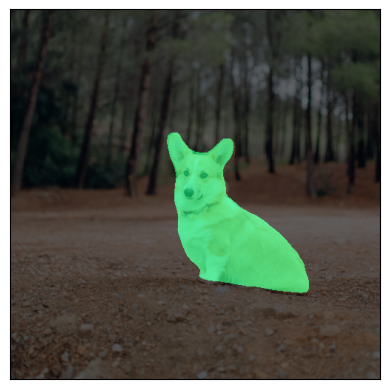
dog_with_all_masks = draw_segmentation_masks(dog1_int, masks=dog1_all_classes_masks, alpha=.6)
show(dog_with_all_masks)

dog1_masks shape = torch.Size([21, 500, 500]), dtype = torch.float32
dog1_all_classes_masks = torch.Size([21, 500, 500]), dtype = torch.bool

我们可以在上图中看到，只绘制了 2 个蒙版：背景蒙版和狗蒙版。这是因为该模型认为只有这两个类在所有像素中是最可能的类。如果该模型检测到另一个类在其他像素中是最可能的类，我们会在上面看到其蒙版。

移除背景蒙版与传递 masks=dog1_all_classes_masks[1:] 一样简单，因为背景类是索引为 0 的类。

现在让我们对整批图像执行相同操作。代码类似，但涉及到对维度进行更多调整。

class_dim = 1
all_classes_masks = normalized_masks.argmax(class_dim) == torch.arange(num_classes)[:, None, None, None]
print(f"shape = {all_classes_masks.shape}, dtype = {all_classes_masks.dtype}")
# The first dimension is the classes now, so we need to swap it
all_classes_masks = all_classes_masks.swapaxes(0, 1)

dogs_with_masks = [
    draw_segmentation_masks(img, masks=mask, alpha=.6)
    for img, mask in zip(dog_list, all_classes_masks)
]
show(dogs_with_masks)

shape = torch.Size([21, 2, 500, 500]), dtype = torch.bool

实例分割模型

实例分割模型的输出与语义分割模型的输出有很大不同。我们将在此处了解如何绘制此类模型的蒙版。我们首先分析 Mask-RCNN 模型的输出。请注意，这些模型不要求图像归一化，因此我们无需使用归一化批处理。

注意

我们在此处将描述 Mask-RCNN 模型的输出。对象检测、实例分割和人员关键点检测 中的模型都具有类似的输出格式，但其中一些模型可能具有额外信息，例如 keypointrcnn_resnet50_fpn() 的关键点，而其中一些模型可能没有蒙版，例如 fasterrcnn_resnet50_fpn()。

from torchvision.models.detection import maskrcnn_resnet50_fpn, MaskRCNN_ResNet50_FPN_Weights

weights = MaskRCNN_ResNet50_FPN_Weights.DEFAULT
transforms = weights.transforms()

images = [transforms(d) for d in dog_list]

model = maskrcnn_resnet50_fpn(weights=weights, progress=False)
model = model.eval()

output = model(images)
print(output)

Downloading: "https://download.pytorch.org/models/maskrcnn_resnet50_fpn_coco-bf2d0c1e.pth" to /root/.cache/torch/hub/checkpoints/maskrcnn_resnet50_fpn_coco-bf2d0c1e.pth
[{'boxes': tensor([[219.7444, 168.1722, 400.7378, 384.0263],
        [343.9716, 171.2287, 358.3447, 222.6263],
        [301.0303, 192.6917, 313.8879, 232.3154]], grad_fn=<StackBackward0>), 'labels': tensor([18,  1,  1]), 'scores': tensor([0.9987, 0.7187, 0.6525], grad_fn=<IndexBackward0>), 'masks': tensor([[[[0., 0., 0.,  ..., 0., 0., 0.],
          [0., 0., 0.,  ..., 0., 0., 0.],
          [0., 0., 0.,  ..., 0., 0., 0.],
          ...,
          [0., 0., 0.,  ..., 0., 0., 0.],
          [0., 0., 0.,  ..., 0., 0., 0.],
          [0., 0., 0.,  ..., 0., 0., 0.]]],


        [[[0., 0., 0.,  ..., 0., 0., 0.],
          [0., 0., 0.,  ..., 0., 0., 0.],
          [0., 0., 0.,  ..., 0., 0., 0.],
          ...,
          [0., 0., 0.,  ..., 0., 0., 0.],
          [0., 0., 0.,  ..., 0., 0., 0.],
          [0., 0., 0.,  ..., 0., 0., 0.]]],


        [[[0., 0., 0.,  ..., 0., 0., 0.],
          [0., 0., 0.,  ..., 0., 0., 0.],
          [0., 0., 0.,  ..., 0., 0., 0.],
          ...,
          [0., 0., 0.,  ..., 0., 0., 0.],
          [0., 0., 0.,  ..., 0., 0., 0.],
          [0., 0., 0.,  ..., 0., 0., 0.]]]], grad_fn=<UnsqueezeBackward0>)}, {'boxes': tensor([[ 44.6767, 137.9018, 446.5324, 487.3429],
        [  0.0000, 288.0053, 489.9292, 490.2352]], grad_fn=<StackBackward0>), 'labels': tensor([18, 15]), 'scores': tensor([0.9978, 0.0697], grad_fn=<IndexBackward0>), 'masks': tensor([[[[0., 0., 0.,  ..., 0., 0., 0.],
          [0., 0., 0.,  ..., 0., 0., 0.],
          [0., 0., 0.,  ..., 0., 0., 0.],
          ...,
          [0., 0., 0.,  ..., 0., 0., 0.],
          [0., 0., 0.,  ..., 0., 0., 0.],
          [0., 0., 0.,  ..., 0., 0., 0.]]],


        [[[0., 0., 0.,  ..., 0., 0., 0.],
          [0., 0., 0.,  ..., 0., 0., 0.],
          [0., 0., 0.,  ..., 0., 0., 0.],
          ...,
          [0., 0., 0.,  ..., 0., 0., 0.],
          [0., 0., 0.,  ..., 0., 0., 0.],
          [0., 0., 0.,  ..., 0., 0., 0.]]]], grad_fn=<UnsqueezeBackward0>)}]

我们来分解一下。对于批处理中的每张图像，模型都会输出一些检测结果（或实例）。每个输入图像的检测结果数量各不相同。每个实例由其边界框、标签、得分和蒙版描述。

输出的组织方式如下：输出是一个长度为 batch_size 的列表。列表中的每个条目对应一个输入图像，它是一个具有键“boxes”、“labels”、“scores”和“masks”的字典。与这些键关联的每个值都有 num_instances 个元素。在上面的示例中，第一个图像中检测到了 3 个实例，第二个图像中检测到了 2 个实例。

可以使用 draw_bounding_boxes() 绘制边框，如上所示，但在这里我们更感兴趣的是掩码。这些掩码与我们上面为语义分割模型看到的掩码有很大不同。

dog1_output = output[0]
dog1_masks = dog1_output['masks']
print(f"shape = {dog1_masks.shape}, dtype = {dog1_masks.dtype}, "
      f"min = {dog1_masks.min()}, max = {dog1_masks.max()}")

shape = torch.Size([3, 1, 500, 500]), dtype = torch.float32, min = 0.0, max = 0.9999862909317017

这里的掩码对应于概率，表示每个像素有多大可能属于该实例的预测标签。这些预测标签对应于同一输出字典中的“labels”元素。让我们看看为第一个图像的实例预测了哪些标签。

print("For the first dog, the following instances were detected:")
print([weights.meta["categories"][label] for label in dog1_output['labels']])

For the first dog, the following instances were detected:
['dog', 'person', 'person']

有趣的是，该模型在图像中检测到了两个人。让我们继续绘制这些掩码。由于 draw_segmentation_masks() 需要布尔掩码，我们需要将这些概率转换为布尔值。请记住，这些掩码的语义是“这个像素有多大可能属于预测的类别？”。因此，将这些掩码转换为布尔值的一种自然方式是对它们使用 0.5 概率进行阈值化（也可以选择不同的阈值）。

proba_threshold = 0.5
dog1_bool_masks = dog1_output['masks'] > proba_threshold
print(f"shape = {dog1_bool_masks.shape}, dtype = {dog1_bool_masks.dtype}")

# There's an extra dimension (1) to the masks. We need to remove it
dog1_bool_masks = dog1_bool_masks.squeeze(1)

show(draw_segmentation_masks(dog1_int, dog1_bool_masks, alpha=0.9))

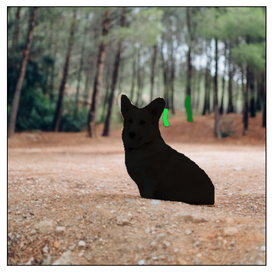
shape = torch.Size([3, 1, 500, 500]), dtype = torch.bool

该模型似乎正确检测到了狗，但它也把树木误认为人。更仔细地查看分数将帮助我们绘制更相关的掩码

print(dog1_output['scores'])

tensor([0.9987, 0.7187, 0.6525], grad_fn=<IndexBackward0>)

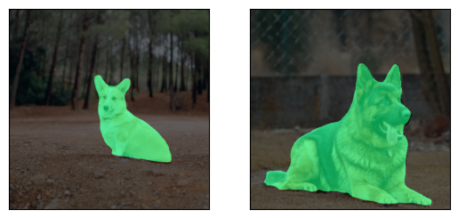
显然，该模型对狗的检测比对人的检测更有信心。这是个好消息。在绘制掩膜时，我们可以只要求得分较高的那些。我们在此使用 0.75 的得分阈值，并绘制第二只狗的掩膜。

score_threshold = .75

boolean_masks = [
    out['masks'][out['scores'] > score_threshold] > proba_threshold
    for out in output
]

dogs_with_masks = [
    draw_segmentation_masks(img, mask.squeeze(1))
    for img, mask in zip(dog_list, boolean_masks)
]
show(dogs_with_masks)

第一张图像中的两个“人”掩膜未被选中，因为它们的分数低于得分阈值。类似地，在第二张图像中，类 15（对应于“长椅”）的实例未被选中。

可视化关键点

可以使用 draw_keypoints() 函数在图像上绘制关键点。我们将看到如何将其与加载了 keypointrcnn_resnet50_fpn() 的 torchvision 的 KeypointRCNN 一起使用。我们首先来看一下模型的输出。

from torchvision.models.detection import keypointrcnn_resnet50_fpn, KeypointRCNN_ResNet50_FPN_Weights
from torchvision.io import read_image

person_int = read_image(str(Path("../assets") / "person1.jpg"))

weights = KeypointRCNN_ResNet50_FPN_Weights.DEFAULT
transforms = weights.transforms()

person_float = transforms(person_int)

model = keypointrcnn_resnet50_fpn(weights=weights, progress=False)
model = model.eval()

outputs = model([person_float])
print(outputs)

Downloading: "https://download.pytorch.org/models/keypointrcnn_resnet50_fpn_coco-fc266e95.pth" to /root/.cache/torch/hub/checkpoints/keypointrcnn_resnet50_fpn_coco-fc266e95.pth
[{'boxes': tensor([[124.3751, 177.9242, 327.6354, 574.7064],
        [124.3625, 180.7574, 290.1061, 390.7958]], grad_fn=<StackBackward0>), 'labels': tensor([1, 1]), 'scores': tensor([0.9998, 0.1070], grad_fn=<IndexBackward0>), 'keypoints': tensor([[[208.0176, 214.2408,   1.0000],
         [208.0176, 207.0375,   1.0000],
         [197.8246, 210.6392,   1.0000],
         [208.0176, 211.8398,   1.0000],
         [178.6378, 217.8425,   1.0000],
         [221.2086, 253.8590,   1.0000],
         [160.6502, 269.4662,   1.0000],
         [243.9929, 304.2822,   1.0000],
         [138.4654, 328.8935,   1.0000],
         [277.5698, 340.8990,   1.0000],
         [153.4551, 374.5144,   1.0000],
         [226.0053, 375.7150,   1.0000],
         [226.0053, 370.3125,   1.0000],
         [221.8082, 455.5516,   1.0000],
         [273.9723, 448.9486,   1.0000],
         [193.6275, 546.1932,   1.0000],
         [273.3727, 545.5930,   1.0000]],

        [[207.8327, 214.6636,   1.0000],
         [207.2343, 207.4622,   1.0000],
         [198.2590, 209.8627,   1.0000],
         [208.4310, 210.4628,   1.0000],
         [178.5134, 218.2642,   1.0000],
         [219.7997, 251.8704,   1.0000],
         [162.3579, 269.2736,   1.0000],
         [245.5289, 304.6800,   1.0000],
         [138.4238, 330.4848,   1.0000],
         [278.4382, 346.0876,   1.0000],
         [153.3826, 374.8929,   1.0000],
         [233.5618, 368.2917,   1.0000],
         [225.7832, 367.6916,   1.0000],
         [289.8069, 357.4897,   1.0000],
         [245.5289, 389.8956,   1.0000],
         [281.4300, 349.0882,   1.0000],
         [209.0294, 389.8956,   1.0000]]], grad_fn=<CopySlices>), 'keypoints_scores': tensor([[16.0164, 16.6672, 15.8312,  4.6510, 14.2053,  8.8280,  9.1136, 12.2084,
         12.1901, 13.8453, 10.7090,  5.5852,  7.5005, 11.3378,  9.3700,  8.2987,
          8.4479],
        [12.9326, 13.8158, 14.9053,  3.9368, 12.9585,  6.4240,  6.8328, 10.4227,
          9.2907, 10.1066, 10.1019,  0.1822,  4.3057, -4.9904, -2.7409, -2.7874,
         -3.9329]], grad_fn=<CopySlices>)}]

正如我们所看到的，输出包含一个字典列表。输出列表的长度为 batch_size。我们目前只有一张图像，因此列表的长度为 1。列表中的每个条目对应于一个输入图像，它是一个字典，键为 boxes、labels、scores、keypoints 和 keypoint_scores。与这些键关联的每个值都包含 num_instances 个元素。在上面的示例中，图像中检测到了 2 个实例。

kpts = outputs[0]['keypoints']
scores = outputs[0]['scores']

print(kpts)
print(scores)

tensor([[[208.0176, 214.2408,   1.0000],
         [208.0176, 207.0375,   1.0000],
         [197.8246, 210.6392,   1.0000],
         [208.0176, 211.8398,   1.0000],
         [178.6378, 217.8425,   1.0000],
         [221.2086, 253.8590,   1.0000],
         [160.6502, 269.4662,   1.0000],
         [243.9929, 304.2822,   1.0000],
         [138.4654, 328.8935,   1.0000],
         [277.5698, 340.8990,   1.0000],
         [153.4551, 374.5144,   1.0000],
         [226.0053, 375.7150,   1.0000],
         [226.0053, 370.3125,   1.0000],
         [221.8082, 455.5516,   1.0000],
         [273.9723, 448.9486,   1.0000],
         [193.6275, 546.1932,   1.0000],
         [273.3727, 545.5930,   1.0000]],

        [[207.8327, 214.6636,   1.0000],
         [207.2343, 207.4622,   1.0000],
         [198.2590, 209.8627,   1.0000],
         [208.4310, 210.4628,   1.0000],
         [178.5134, 218.2642,   1.0000],
         [219.7997, 251.8704,   1.0000],
         [162.3579, 269.2736,   1.0000],
         [245.5289, 304.6800,   1.0000],
         [138.4238, 330.4848,   1.0000],
         [278.4382, 346.0876,   1.0000],
         [153.3826, 374.8929,   1.0000],
         [233.5618, 368.2917,   1.0000],
         [225.7832, 367.6916,   1.0000],
         [289.8069, 357.4897,   1.0000],
         [245.5289, 389.8956,   1.0000],
         [281.4300, 349.0882,   1.0000],
         [209.0294, 389.8956,   1.0000]]], grad_fn=<CopySlices>)
tensor([0.9998, 0.1070], grad_fn=<IndexBackward0>)

KeypointRCNN 模型检测到图像中有两个实例。如果你使用 draw_bounding_boxes() 绘制边框，你会发现它们是人冲浪板。如果我们查看分数，我们会发现模型对人的信心比对冲浪板的信心大得多。我们现在可以设置一个阈值置信度，并绘制我们有足够信心的实例。我们设置一个 0.75 的阈值，并过滤掉对应于人的关键点。

detect_threshold = 0.75
idx = torch.where(scores > detect_threshold)
keypoints = kpts[idx]

print(keypoints)

tensor([[[208.0176, 214.2408,   1.0000],
         [208.0176, 207.0375,   1.0000],
         [197.8246, 210.6392,   1.0000],
         [208.0176, 211.8398,   1.0000],
         [178.6378, 217.8425,   1.0000],
         [221.2086, 253.8590,   1.0000],
         [160.6502, 269.4662,   1.0000],
         [243.9929, 304.2822,   1.0000],
         [138.4654, 328.8935,   1.0000],
         [277.5698, 340.8990,   1.0000],
         [153.4551, 374.5144,   1.0000],
         [226.0053, 375.7150,   1.0000],
         [226.0053, 370.3125,   1.0000],
         [221.8082, 455.5516,   1.0000],
         [273.9723, 448.9486,   1.0000],
         [193.6275, 546.1932,   1.0000],
         [273.3727, 545.5930,   1.0000]]], grad_fn=<IndexBackward0>)

太棒了，现在我们有了对应于人的关键点。每个关键点由 x、y 坐标和可见性表示。我们现在可以使用 draw_keypoints() 函数绘制关键点。请注意，该实用程序需要 uint8 图像。

from torchvision.utils import draw_keypoints

res = draw_keypoints(person_int, keypoints, colors="blue", radius=3)
show(res)

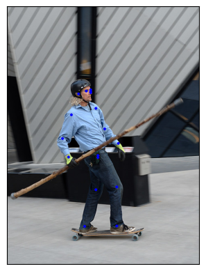
正如我们所看到的，关键点显示为图像上的彩色圆圈。人的 coco 关键点是有序的，表示以下列表。

coco_keypoints = [
    "nose", "left_eye", "right_eye", "left_ear", "right_ear",
    "left_shoulder", "right_shoulder", "left_elbow", "right_elbow",
    "left_wrist", "right_wrist", "left_hip", "right_hip",
    "left_knee", "right_knee", "left_ankle", "right_ankle",
]

如果我们有兴趣连接关键点怎么办？这在创建姿势检测或动作识别时特别有用。我们可以使用 connectivity 参数轻松连接关键点。仔细观察会发现，我们需要按以下顺序连接点才能构建人体骨架。

鼻子 -> 左眼 -> 左耳。（0, 1）、（1, 3）

鼻子 -> 右眼 -> 右耳。(0, 2)，(2, 4)

鼻子 -> 左肩 -> 左肘 -> 左腕。(0, 5)，(5, 7)，(7, 9)

鼻子 -> 右肩 -> 右肘 -> 右腕。(0, 6)，(6, 8)，(8, 10)

左肩 -> 左髋 -> 左膝 -> 左脚踝。(5, 11)，(11, 13)，(13, 15)

右肩 -> 右髋 -> 右膝 -> 右脚踝。(6, 12)，(12, 14)，(14, 16)

我们将创建一个包含这些关键点 ID 的列表，以进行连接。

connect_skeleton = [
    (0, 1), (0, 2), (1, 3), (2, 4), (0, 5), (0, 6), (5, 7), (6, 8),
    (7, 9), (8, 10), (5, 11), (6, 12), (11, 13), (12, 14), (13, 15), (14, 16)
]

我们将上述列表传递给连接参数以连接关键点。

res = draw_keypoints(person_int, keypoints, connectivity=connect_skeleton, colors="blue", radius=4, width=3)
show(res)

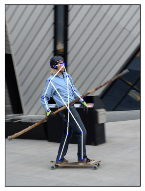
看起来相当不错。

绘制具有可见性的关键点

让我们看看结果，另一个关键点预测模块生成并显示连接

prediction = torch.tensor(
    [[[208.0176, 214.2409, 1.0000],
      [000.0000, 000.0000, 0.0000],
      [197.8246, 210.6392, 1.0000],
      [000.0000, 000.0000, 0.0000],
      [178.6378, 217.8425, 1.0000],
      [221.2086, 253.8591, 1.0000],
      [160.6502, 269.4662, 1.0000],
      [243.9929, 304.2822, 1.0000],
      [138.4654, 328.8935, 1.0000],
      [277.5698, 340.8990, 1.0000],
      [153.4551, 374.5145, 1.0000],
      [000.0000, 000.0000, 0.0000],
      [226.0053, 370.3125, 1.0000],
      [221.8081, 455.5516, 1.0000],
      [273.9723, 448.9486, 1.0000],
      [193.6275, 546.1933, 1.0000],
      [273.3727, 545.5930, 1.0000]]]
)

res = draw_keypoints(person_int, prediction, connectivity=connect_skeleton, colors="blue", radius=4, width=3)
show(res)

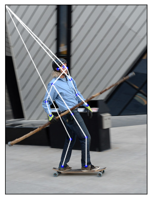
那里发生了什么？预测新关键点的模型无法检测到滑板运动员左上半身隐藏的三个点。更准确地说，该模型预测左眼、左耳和左髋的 (x, y, vis) = (0, 0, 0)。因此，我们肯定不想显示这些关键点和连接，而且您也不必这样做。查看 draw_keypoints() 的参数，我们可以看到可以将可见性张量作为附加参数传递。鉴于模型的预测，我们具有可见性作为第三个关键点维度，我们只需要提取它。让我们将 prediction 分割为关键点坐标及其各自的可见性，并将两者作为参数传递给 draw_keypoints()。

coordinates, visibility = prediction.split([2, 1], dim=-1)
visibility = visibility.bool()

res = draw_keypoints(
    person_int, coordinates, visibility=visibility, connectivity=connect_skeleton, colors="blue", radius=4, width=3
)
show(res)

我们可以看到未检测到的关键点没有绘制，并且跳过了不可见的关键点连接。这可以减少具有多个检测的图像上的噪声，或者在像我们这样的情况下，当关键点预测模型错过一些检测时。大多数火炬关键点预测模型都会返回每个预测的可见性，以便您随时使用。我们第一个案例中使用的keypointrcnn_resnet50_fpn()模型也这样做。