


注意
单击 这里 下载完整的示例代码
使用 CTC 解码器的 ASR 推理
作者: Caroline Chen
本教程演示了如何使用具有词典约束和 KenLM 语言模型支持的 CTC 光束搜索解码器执行语音识别推理。我们将在使用 CTC 损失训练的预训练 wav2vec 2.0 模型上演示这一点。
概述
光束搜索解码通过迭代地扩展文本假设(光束)并添加下一个可能的字符来工作,并且在每个时间步只保留得分最高的假设。语言模型可以集成到评分计算中,并且添加词典约束可以限制假设的下一个可能标记,以使只有来自词典的单词可以生成。
底层实现是从 Flashlight 的光束搜索解码器移植的。解码器优化的数学公式可以在 Wav2Letter 论文 中找到,更详细的算法可以在这个 博客 中找到。
使用具有语言模型和词典约束的 CTC 光束搜索解码器运行 ASR 推理需要以下组件
声学模型:从音频波形预测语音的模型
标记:声学模型可以预测的可能标记
词典:可能单词与其对应的标记序列之间的映射
语言模型 (LM):使用 KenLM 库 训练的 N 元语言模型,或继承
CTCDecoderLM的自定义语言模型
声学模型和设置
首先,我们导入必要的实用程序并获取我们正在处理的数据
import torch
import torchaudio

print(torch.__version__)
print(torchaudio.__version__)
2.4.0
2.4.0
import time
from typing import List

import IPython
import matplotlib.pyplot as plt
from torchaudio.models.decoder import ctc_decoder
from torchaudio.utils import download_asset
我们使用在 Wav2Vec 2.0 基础模型上微调的预训练模型,该模型在 LibriSpeech 数据集 的 10 分钟数据上进行了微调,可以使用 torchaudio.pipelines.WAV2VEC2_ASR_BASE_10M 加载。有关在 torchaudio 中运行 Wav2Vec 2.0 语音识别管道的更多详细信息,请参阅 本教程。
bundle = torchaudio.pipelines.WAV2VEC2_ASR_BASE_10M
acoustic_model = bundle.get_model()
Downloading: "https://download.pytorch.org/torchaudio/models/wav2vec2_fairseq_base_ls960_asr_ll10m.pth" to /root/.cache/torch/hub/checkpoints/wav2vec2_fairseq_base_ls960_asr_ll10m.pth

  0%|          | 0.00/360M [00:00<?, ?B/s]
  4%|4         | 15.8M/360M [00:00<00:02, 123MB/s]
  8%|7         | 27.5M/360M [00:00<00:04, 86.5MB/s]
 10%|#         | 36.1M/360M [00:00<00:05, 66.8MB/s]
 13%|#3        | 46.9M/360M [00:00<00:04, 72.7MB/s]
 15%|#5        | 54.2M/360M [00:00<00:04, 65.2MB/s]
 18%|#7        | 64.0M/360M [00:00<00:04, 62.3MB/s]
 22%|##2       | 79.8M/360M [00:01<00:03, 78.7MB/s]
 24%|##4       | 87.6M/360M [00:01<00:03, 73.2MB/s]
 27%|##6       | 95.8M/360M [00:01<00:03, 74.5MB/s]
 29%|##8       | 103M/360M [00:01<00:04, 63.6MB/s]
 31%|###       | 111M/360M [00:01<00:03, 65.7MB/s]
 33%|###2      | 117M/360M [00:01<00:04, 62.8MB/s]
 35%|###5      | 127M/360M [00:01<00:03, 67.1MB/s]
 37%|###7      | 133M/360M [00:02<00:04, 49.4MB/s]
 40%|###9      | 144M/360M [00:02<00:04, 49.8MB/s]
 41%|####1     | 149M/360M [00:02<00:04, 45.8MB/s]
 43%|####2     | 154M/360M [00:02<00:05, 39.9MB/s]
 44%|####4     | 160M/360M [00:02<00:05, 41.5MB/s]
 49%|####8     | 175M/360M [00:03<00:03, 52.2MB/s]
 50%|####9     | 180M/360M [00:03<00:04, 42.5MB/s]
 53%|#####3    | 192M/360M [00:03<00:03, 53.5MB/s]
 58%|#####7    | 208M/360M [00:03<00:02, 61.5MB/s]
 62%|######2   | 224M/360M [00:03<00:02, 65.0MB/s]
 67%|######6   | 240M/360M [00:04<00:02, 57.0MB/s]
 68%|######8   | 246M/360M [00:04<00:02, 44.7MB/s]
 71%|#######1  | 256M/360M [00:04<00:02, 45.2MB/s]
 72%|#######2  | 260M/360M [00:04<00:02, 43.1MB/s]
 76%|#######5  | 272M/360M [00:05<00:01, 49.7MB/s]
 80%|#######9  | 287M/360M [00:05<00:01, 68.8MB/s]
 82%|########2 | 296M/360M [00:05<00:01, 61.2MB/s]
 84%|########4 | 303M/360M [00:05<00:01, 58.5MB/s]
 86%|########5 | 309M/360M [00:05<00:01, 46.7MB/s]
 89%|########8 | 319M/360M [00:05<00:00, 49.8MB/s]
 90%|######### | 324M/360M [00:06<00:00, 46.0MB/s]
 93%|#########3| 336M/360M [00:06<00:00, 56.9MB/s]
 98%|#########7| 352M/360M [00:06<00:00, 68.7MB/s]
100%|##########| 360M/360M [00:06<00:00, 58.6MB/s]
我们将从 LibriSpeech test-other 数据集中加载一个样本。
speech_file = download_asset("tutorial-assets/ctc-decoding/1688-142285-0007.wav")

IPython.display.Audio(speech_file)
与该音频文件对应的转录本为
waveform, sample_rate = torchaudio.load(speech_file)

if sample_rate != bundle.sample_rate:
    waveform = torchaudio.functional.resample(waveform, sample_rate, bundle.sample_rate)
解码器文件和数据
接下来,我们加载我们的标记、词典和语言模型数据,这些数据由解码器用于从声学模型输出预测单词。LibriSpeech 数据集的预训练文件可以通过 torchaudio 下载,或者用户可以提供自己的文件。
标记
标记是声学模型可以预测的可能符号,包括空格和静音符号。它可以作为文件传入,其中每行包含与同一索引对应的标记,也可以作为标记列表传入,每个标记映射到一个唯一的索引。
# tokens.txt
_
|
e
t
...
['-', '|', 'e', 't', 'a', 'o', 'n', 'i', 'h', 's', 'r', 'd', 'l', 'u', 'm', 'w', 'c', 'f', 'g', 'y', 'p', 'b', 'v', 'k', "'", 'x', 'j', 'q', 'z']
词典
词典是单词与其对应的标记序列之间的映射,用于将解码器的搜索空间限制为词典中的单词。词典文件的预期格式是每个单词一行,一个单词后跟其空格分隔的标记。
# lexcion.txt
a a |
able a b l e |
about a b o u t |
...
...
语言模型
语言模型可以在解码中使用,通过将表示序列可能性的语言模型得分考虑进光束搜索计算来提高结果。下面,我们概述了支持解码的不同形式的语言模型。
没有语言模型
要创建没有语言模型的解码器实例,在初始化解码器时将 lm=None 设置为。
KenLM
这是一个使用 KenLM 库 训练的 N 元语言模型。可以使用 .arpa 或二进制化 .bin LM,但建议使用二进制格式,因为它加载速度更快。
本教程中使用的语言模型是使用 LibriSpeech 训练的 4 元 KenLM。
自定义语言模型
用户可以使用 Python 定义自己的自定义语言模型,无论是统计语言模型还是神经网络语言模型,都可以使用 CTCDecoderLM 和 CTCDecoderLMState。
例如,以下代码创建了一个围绕 PyTorch torch.nn.Module 语言模型的基本包装器。
from torchaudio.models.decoder import CTCDecoderLM, CTCDecoderLMState


class CustomLM(CTCDecoderLM):
    """Create a Python wrapper around `language_model` to feed to the decoder."""

    def __init__(self, language_model: torch.nn.Module):
        CTCDecoderLM.__init__(self)
        self.language_model = language_model
        self.sil = -1  # index for silent token in the language model
        self.states = {}

        language_model.eval()

    def start(self, start_with_nothing: bool = False):
        state = CTCDecoderLMState()
        with torch.no_grad():
            score = self.language_model(self.sil)

        self.states[state] = score
        return state

    def score(self, state: CTCDecoderLMState, token_index: int):
        outstate = state.child(token_index)
        if outstate not in self.states:
            score = self.language_model(token_index)
            self.states[outstate] = score
        score = self.states[outstate]

        return outstate, score

    def finish(self, state: CTCDecoderLMState):
        return self.score(state, self.sil)
下载预训练文件
可以使用 download_pretrained_files() 下载 LibriSpeech 数据集的预训练文件。
注意:由于语言模型可能很大,此单元格可能需要几分钟才能运行。
from torchaudio.models.decoder import download_pretrained_files

files = download_pretrained_files("librispeech-4-gram")

print(files)
  0%|          | 0.00/4.97M [00:00<?, ?B/s]
 85%|########5 | 4.25M/4.97M [00:00<00:00, 20.0MB/s]
100%|##########| 4.97M/4.97M [00:00<00:00, 22.9MB/s]

  0%|          | 0.00/57.0 [00:00<?, ?B/s]
100%|##########| 57.0/57.0 [00:00<00:00, 56.3kB/s]

  0%|          | 0.00/2.91G [00:00<?, ?B/s]
  0%|          | 14.9M/2.91G [00:00<01:01, 50.5MB/s]
  1%|          | 19.8M/2.91G [00:00<01:04, 48.3MB/s]
  1%|1         | 32.0M/2.91G [00:00<00:50, 61.8MB/s]
  2%|1         | 46.9M/2.91G [00:00<00:42, 72.6MB/s]
  2%|1         | 53.9M/2.91G [00:00<00:43, 69.8MB/s]
  2%|2         | 62.9M/2.91G [00:00<00:41, 73.0MB/s]
  2%|2         | 69.9M/2.91G [00:01<00:52, 57.9MB/s]
  3%|2         | 79.8M/2.91G [00:01<00:46, 65.8MB/s]
  3%|2         | 86.5M/2.91G [00:01<00:52, 57.4MB/s]
  3%|3         | 94.9M/2.91G [00:01<00:54, 55.2MB/s]
  3%|3         | 100M/2.91G [00:01<01:02, 48.6MB/s]
  4%|3         | 112M/2.91G [00:01<00:50, 59.5MB/s]
  4%|4         | 128M/2.91G [00:02<00:43, 69.1MB/s]
  5%|4         | 144M/2.91G [00:02<00:42, 70.3MB/s]
  5%|5         | 159M/2.91G [00:02<00:41, 71.9MB/s]
  6%|5         | 166M/2.91G [00:02<00:47, 62.2MB/s]
  6%|5         | 176M/2.91G [00:02<00:42, 69.8MB/s]
  6%|6         | 192M/2.91G [00:03<00:41, 71.3MB/s]
  7%|6         | 208M/2.91G [00:03<00:43, 66.1MB/s]
  8%|7         | 224M/2.91G [00:03<00:51, 56.4MB/s]
  8%|7         | 230M/2.91G [00:03<00:52, 55.0MB/s]
  8%|8         | 240M/2.91G [00:04<00:51, 56.0MB/s]
  9%|8         | 255M/2.91G [00:04<00:41, 68.6MB/s]
  9%|8         | 262M/2.91G [00:04<00:46, 61.5MB/s]
  9%|9         | 272M/2.91G [00:04<00:48, 58.3MB/s]
  9%|9         | 281M/2.91G [00:04<00:43, 64.5MB/s]
 10%|9         | 288M/2.91G [00:04<00:44, 63.6MB/s]
 10%|#         | 299M/2.91G [00:04<00:38, 73.9MB/s]
 10%|#         | 306M/2.91G [00:05<01:00, 46.4MB/s]
 11%|#         | 319M/2.91G [00:05<00:49, 56.7MB/s]
 11%|#         | 326M/2.91G [00:05<00:53, 51.9MB/s]
 11%|#1        | 336M/2.91G [00:05<00:50, 54.9MB/s]
 12%|#1        | 352M/2.91G [00:06<00:53, 51.3MB/s]
 12%|#2        | 367M/2.91G [00:06<00:47, 57.4MB/s]
 13%|#2        | 373M/2.91G [00:06<00:57, 47.2MB/s]
 13%|#2        | 384M/2.91G [00:06<00:54, 50.2MB/s]
 13%|#3        | 400M/2.91G [00:06<00:43, 62.2MB/s]
 14%|#3        | 416M/2.91G [00:07<00:40, 66.3MB/s]
 14%|#4        | 432M/2.91G [00:07<00:38, 68.9MB/s]
 15%|#4        | 439M/2.91G [00:07<00:42, 62.5MB/s]
 15%|#5        | 448M/2.91G [00:07<00:50, 52.8MB/s]
 15%|#5        | 453M/2.91G [00:08<01:01, 43.0MB/s]
 16%|#5        | 464M/2.91G [00:08<00:58, 44.9MB/s]
 16%|#6        | 480M/2.91G [00:08<00:47, 55.4MB/s]
 17%|#6        | 496M/2.91G [00:08<00:42, 61.8MB/s]
 17%|#6        | 502M/2.91G [00:08<00:48, 53.1MB/s]
 17%|#7        | 511M/2.91G [00:09<00:44, 58.3MB/s]
 17%|#7        | 517M/2.91G [00:09<00:49, 52.6MB/s]
 18%|#7        | 527M/2.91G [00:09<01:09, 37.1MB/s]
 18%|#7        | 531M/2.91G [00:09<01:07, 38.2MB/s]
 18%|#8        | 544M/2.91G [00:09<00:51, 49.1MB/s]
 19%|#8        | 559M/2.91G [00:10<00:50, 50.5MB/s]
 19%|#8        | 564M/2.91G [00:10<00:58, 43.4MB/s]
 19%|#9        | 575M/2.91G [00:10<00:54, 46.4MB/s]
 19%|#9        | 580M/2.91G [00:10<00:58, 42.8MB/s]
 20%|#9        | 592M/2.91G [00:11<00:53, 47.1MB/s]
 20%|##        | 607M/2.91G [00:11<00:44, 56.3MB/s]
 21%|##        | 612M/2.91G [00:11<00:52, 47.4MB/s]
 21%|##        | 623M/2.91G [00:11<00:46, 53.7MB/s]
 21%|##1       | 628M/2.91G [00:11<00:52, 47.3MB/s]
 21%|##1       | 639M/2.91G [00:11<00:44, 55.7MB/s]
 22%|##1       | 644M/2.91G [00:12<00:47, 51.9MB/s]
 22%|##2       | 656M/2.91G [00:12<00:44, 55.4MB/s]
 23%|##2       | 672M/2.91G [00:12<00:38, 62.4MB/s]
 23%|##2       | 678M/2.91G [00:12<00:56, 43.0MB/s]
 23%|##3       | 688M/2.91G [00:13<00:53, 45.0MB/s]
 23%|##3       | 692M/2.91G [00:13<00:53, 44.5MB/s]
 23%|##3       | 698M/2.91G [00:13<00:51, 46.3MB/s]
 24%|##3       | 704M/2.91G [00:13<00:58, 40.8MB/s]
 24%|##3       | 715M/2.91G [00:13<00:43, 55.0MB/s]
 24%|##4       | 721M/2.91G [00:13<00:52, 44.7MB/s]
 25%|##4       | 731M/2.91G [00:13<00:48, 49.1MB/s]
 25%|##4       | 736M/2.91G [00:14<00:53, 43.8MB/s]
 25%|##5       | 749M/2.91G [00:14<00:38, 61.5MB/s]
 25%|##5       | 756M/2.91G [00:14<00:41, 55.9MB/s]
 26%|##5       | 768M/2.91G [00:14<00:39, 58.6MB/s]
 26%|##6       | 784M/2.91G [00:14<00:31, 73.2MB/s]
 27%|##6       | 799M/2.91G [00:14<00:27, 83.7MB/s]
 27%|##7       | 807M/2.91G [00:15<00:36, 62.0MB/s]
 27%|##7       | 815M/2.91G [00:15<00:37, 60.2MB/s]
 28%|##7       | 821M/2.91G [00:15<00:38, 59.2MB/s]
 28%|##7       | 831M/2.91G [00:15<00:34, 65.2MB/s]
 28%|##8       | 838M/2.91G [00:15<00:41, 54.2MB/s]
 28%|##8       | 848M/2.91G [00:15<00:36, 61.0MB/s]
 29%|##8       | 864M/2.91G [00:16<00:32, 69.0MB/s]
 30%|##9       | 880M/2.91G [00:16<00:24, 88.2MB/s]
 30%|##9       | 889M/2.91G [00:16<00:35, 62.5MB/s]
 30%|###       | 897M/2.91G [00:16<00:40, 54.3MB/s]
 31%|###       | 912M/2.91G [00:16<00:30, 70.3MB/s]
 31%|###       | 920M/2.91G [00:17<00:33, 65.0MB/s]
 31%|###1      | 928M/2.91G [00:17<00:37, 57.0MB/s]
 31%|###1      | 934M/2.91G [00:17<00:41, 51.9MB/s]
 32%|###1      | 944M/2.91G [00:17<00:43, 48.9MB/s]
 32%|###2      | 960M/2.91G [00:17<00:44, 47.3MB/s]
 32%|###2      | 965M/2.91G [00:18<00:47, 44.1MB/s]
 33%|###2      | 975M/2.91G [00:18<00:44, 47.8MB/s]
 33%|###2      | 980M/2.91G [00:18<00:50, 41.3MB/s]
 33%|###3      | 992M/2.91G [00:18<00:42, 49.3MB/s]
 34%|###3      | 0.98G/2.91G [00:18<00:33, 62.1MB/s]
 34%|###4      | 1.00G/2.91G [00:18<00:26, 77.4MB/s]
 35%|###4      | 1.01G/2.91G [00:19<00:32, 62.7MB/s]
 35%|###4      | 1.02G/2.91G [00:19<00:32, 63.1MB/s]
 35%|###5      | 1.02G/2.91G [00:19<00:34, 59.3MB/s]
 35%|###5      | 1.03G/2.91G [00:19<00:34, 58.7MB/s]
 36%|###5      | 1.04G/2.91G [00:19<00:28, 71.6MB/s]
 36%|###6      | 1.05G/2.91G [00:19<00:29, 67.1MB/s]
 37%|###6      | 1.06G/2.91G [00:20<00:28, 70.4MB/s]
 37%|###7      | 1.08G/2.91G [00:20<00:26, 74.6MB/s]
 38%|###7      | 1.09G/2.91G [00:20<00:26, 73.8MB/s]
 38%|###8      | 1.11G/2.91G [00:20<00:25, 75.2MB/s]
 39%|###8      | 1.12G/2.91G [00:20<00:25, 74.0MB/s]
 39%|###8      | 1.13G/2.91G [00:21<00:28, 67.4MB/s]
 39%|###9      | 1.14G/2.91G [00:21<00:32, 57.9MB/s]
 40%|###9      | 1.16G/2.91G [00:21<00:27, 69.8MB/s]
 40%|###9      | 1.16G/2.91G [00:21<00:32, 57.1MB/s]
 40%|####      | 1.17G/2.91G [00:21<00:30, 61.0MB/s]
 41%|####      | 1.19G/2.91G [00:22<00:28, 65.0MB/s]
 41%|####1     | 1.20G/2.91G [00:22<00:25, 70.5MB/s]
 42%|####1     | 1.22G/2.91G [00:22<00:20, 87.0MB/s]
 42%|####2     | 1.23G/2.91G [00:22<00:21, 82.5MB/s]
 42%|####2     | 1.24G/2.91G [00:22<00:30, 58.1MB/s]
 43%|####2     | 1.25G/2.91G [00:23<00:27, 64.3MB/s]
 43%|####3     | 1.26G/2.91G [00:23<00:27, 65.3MB/s]
 43%|####3     | 1.27G/2.91G [00:23<00:27, 64.2MB/s]
 44%|####4     | 1.28G/2.91G [00:23<00:24, 70.8MB/s]
 45%|####4     | 1.30G/2.91G [00:23<00:22, 77.3MB/s]
 45%|####4     | 1.30G/2.91G [00:23<00:25, 68.7MB/s]
 45%|####5     | 1.31G/2.91G [00:24<00:26, 65.6MB/s]
 45%|####5     | 1.32G/2.91G [00:24<00:30, 56.9MB/s]
 46%|####5     | 1.33G/2.91G [00:24<00:32, 52.0MB/s]
 46%|####6     | 1.34G/2.91G [00:24<00:25, 64.9MB/s]
 46%|####6     | 1.35G/2.91G [00:24<00:29, 57.6MB/s]
 47%|####6     | 1.36G/2.91G [00:24<00:24, 66.8MB/s]
 47%|####6     | 1.37G/2.91G [00:24<00:25, 65.7MB/s]
 47%|####7     | 1.38G/2.91G [00:25<00:27, 60.8MB/s]
 48%|####7     | 1.39G/2.91G [00:25<00:25, 62.8MB/s]
 48%|####7     | 1.40G/2.91G [00:25<00:30, 53.7MB/s]
 48%|####8     | 1.41G/2.91G [00:25<00:24, 66.0MB/s]
 49%|####8     | 1.42G/2.91G [00:25<00:22, 72.6MB/s]
 49%|####9     | 1.44G/2.91G [00:26<00:19, 79.3MB/s]
 50%|####9     | 1.45G/2.91G [00:26<00:20, 75.2MB/s]
 50%|#####     | 1.46G/2.91G [00:26<00:25, 62.2MB/s]
 50%|#####     | 1.47G/2.91G [00:26<00:26, 58.9MB/s]
 51%|#####     | 1.47G/2.91G [00:27<00:40, 38.5MB/s]
 51%|#####1    | 1.48G/2.91G [00:27<00:35, 43.6MB/s]
 51%|#####1    | 1.49G/2.91G [00:27<00:41, 37.1MB/s]
 52%|#####1    | 1.50G/2.91G [00:27<00:37, 40.1MB/s]
 52%|#####1    | 1.50G/2.91G [00:28<00:44, 33.6MB/s]
 52%|#####2    | 1.51G/2.91G [00:28<00:33, 44.6MB/s]
 52%|#####2    | 1.52G/2.91G [00:28<00:34, 43.1MB/s]
 52%|#####2    | 1.52G/2.91G [00:28<00:33, 43.9MB/s]
 53%|#####2    | 1.53G/2.91G [00:28<00:35, 41.2MB/s]
 53%|#####2    | 1.53G/2.91G [00:28<00:45, 32.8MB/s]
 53%|#####3    | 1.55G/2.91G [00:28<00:35, 41.7MB/s]
 53%|#####3    | 1.55G/2.91G [00:29<00:33, 43.4MB/s]
 54%|#####3    | 1.56G/2.91G [00:29<00:26, 55.5MB/s]
 54%|#####4    | 1.58G/2.91G [00:29<00:21, 65.2MB/s]
 55%|#####4    | 1.59G/2.91G [00:29<00:17, 82.7MB/s]
 55%|#####5    | 1.60G/2.91G [00:29<00:19, 71.5MB/s]
 55%|#####5    | 1.61G/2.91G [00:29<00:23, 60.2MB/s]
 56%|#####5    | 1.62G/2.91G [00:30<00:20, 68.7MB/s]
 56%|#####6    | 1.64G/2.91G [00:30<00:18, 75.7MB/s]
 57%|#####6    | 1.65G/2.91G [00:30<00:29, 46.7MB/s]
 57%|#####6    | 1.66G/2.91G [00:30<00:30, 44.5MB/s]
 57%|#####7    | 1.66G/2.91G [00:31<00:29, 45.0MB/s]
 57%|#####7    | 1.67G/2.91G [00:31<00:27, 47.8MB/s]
 58%|#####7    | 1.68G/2.91G [00:31<00:31, 41.6MB/s]
 58%|#####7    | 1.69G/2.91G [00:31<00:26, 49.4MB/s]
 59%|#####8    | 1.70G/2.91G [00:31<00:19, 66.1MB/s]
 59%|#####9    | 1.72G/2.91G [00:31<00:17, 74.2MB/s]
 60%|#####9    | 1.73G/2.91G [00:32<00:14, 86.5MB/s]
 60%|#####9    | 1.74G/2.91G [00:32<00:19, 63.2MB/s]
 60%|######    | 1.75G/2.91G [00:32<00:24, 50.4MB/s]
 60%|######    | 1.76G/2.91G [00:32<00:28, 44.0MB/s]
 61%|######    | 1.76G/2.91G [00:33<00:27, 45.2MB/s]
 61%|######    | 1.77G/2.91G [00:33<00:35, 34.9MB/s]
 61%|######1   | 1.78G/2.91G [00:33<00:30, 40.1MB/s]
 61%|######1   | 1.79G/2.91G [00:33<00:29, 40.4MB/s]
 62%|######1   | 1.80G/2.91G [00:33<00:23, 50.5MB/s]
 62%|######2   | 1.81G/2.91G [00:34<00:19, 60.3MB/s]
 62%|######2   | 1.82G/2.91G [00:34<00:19, 60.5MB/s]
 63%|######2   | 1.82G/2.91G [00:34<00:23, 49.1MB/s]
 63%|######2   | 1.83G/2.91G [00:34<00:30, 37.8MB/s]
 63%|######3   | 1.84G/2.91G [00:34<00:23, 49.3MB/s]
 64%|######3   | 1.86G/2.91G [00:35<00:19, 56.6MB/s]
 64%|######4   | 1.87G/2.91G [00:35<00:15, 72.2MB/s]
 65%|######4   | 1.88G/2.91G [00:35<00:17, 64.7MB/s]
 65%|######4   | 1.89G/2.91G [00:35<00:18, 58.0MB/s]
 65%|######5   | 1.91G/2.91G [00:35<00:18, 57.4MB/s]
 66%|######5   | 1.91G/2.91G [00:36<00:20, 51.1MB/s]
 66%|######6   | 1.92G/2.91G [00:36<00:20, 52.0MB/s]
 67%|######6   | 1.94G/2.91G [00:36<00:15, 66.8MB/s]
 67%|######6   | 1.94G/2.91G [00:36<00:17, 59.6MB/s]
 67%|######7   | 1.95G/2.91G [00:36<00:16, 62.1MB/s]
 67%|######7   | 1.96G/2.91G [00:36<00:18, 55.0MB/s]
 68%|######7   | 1.97G/2.91G [00:37<00:18, 54.4MB/s]
 68%|######7   | 1.97G/2.91G [00:37<00:23, 42.9MB/s]
 68%|######7   | 1.98G/2.91G [00:37<00:24, 40.8MB/s]
 68%|######8   | 1.98G/2.91G [00:37<00:27, 36.5MB/s]
 68%|######8   | 1.99G/2.91G [00:37<00:26, 37.3MB/s]
 69%|######8   | 2.00G/2.91G [00:38<00:26, 37.4MB/s]
 69%|######9   | 2.01G/2.91G [00:38<00:18, 53.1MB/s]
 69%|######9   | 2.02G/2.91G [00:38<00:19, 49.3MB/s]
 70%|######9   | 2.03G/2.91G [00:38<00:16, 58.9MB/s]
 70%|######9   | 2.04G/2.91G [00:38<00:16, 55.5MB/s]
 70%|#######   | 2.05G/2.91G [00:38<00:16, 56.0MB/s]
 70%|#######   | 2.05G/2.91G [00:39<00:18, 48.7MB/s]
 71%|#######   | 2.06G/2.91G [00:39<00:15, 60.3MB/s]
 71%|#######1  | 2.07G/2.91G [00:39<00:18, 49.2MB/s]
 71%|#######1  | 2.08G/2.91G [00:39<00:18, 48.4MB/s]
 72%|#######1  | 2.09G/2.91G [00:39<00:14, 60.7MB/s]
 72%|#######2  | 2.11G/2.91G [00:39<00:12, 71.0MB/s]
 73%|#######2  | 2.12G/2.91G [00:40<00:13, 63.5MB/s]
 73%|#######3  | 2.12G/2.91G [00:40<00:14, 59.1MB/s]
 74%|#######3  | 2.14G/2.91G [00:40<00:12, 68.1MB/s]
 74%|#######4  | 2.16G/2.91G [00:40<00:10, 77.0MB/s]
 74%|#######4  | 2.16G/2.91G [00:40<00:10, 76.2MB/s]
 75%|#######4  | 2.17G/2.91G [00:40<00:12, 66.2MB/s]
 75%|#######4  | 2.18G/2.91G [00:41<00:10, 73.2MB/s]
 75%|#######5  | 2.19G/2.91G [00:41<00:14, 54.8MB/s]
 76%|#######5  | 2.20G/2.91G [00:41<00:10, 74.5MB/s]
 76%|#######6  | 2.22G/2.91G [00:41<00:10, 70.5MB/s]
 77%|#######6  | 2.23G/2.91G [00:41<00:10, 69.9MB/s]
 77%|#######6  | 2.24G/2.91G [00:42<00:14, 49.7MB/s]
 77%|#######7  | 2.25G/2.91G [00:42<00:13, 52.5MB/s]
 77%|#######7  | 2.25G/2.91G [00:42<00:14, 49.8MB/s]
 78%|#######7  | 2.27G/2.91G [00:42<00:11, 58.0MB/s]
 78%|#######8  | 2.28G/2.91G [00:42<00:09, 72.6MB/s]
 79%|#######8  | 2.29G/2.91G [00:43<00:12, 54.4MB/s]
 79%|#######8  | 2.30G/2.91G [00:43<00:13, 47.5MB/s]
 79%|#######9  | 2.30G/2.91G [00:43<00:15, 41.6MB/s]
 79%|#######9  | 2.31G/2.91G [00:43<00:13, 49.1MB/s]
 80%|#######9  | 2.32G/2.91G [00:43<00:10, 62.1MB/s]
 80%|########  | 2.33G/2.91G [00:44<00:16, 37.2MB/s]
 81%|########  | 2.34G/2.91G [00:44<00:14, 41.9MB/s]
 81%|########  | 2.35G/2.91G [00:44<00:16, 36.4MB/s]
 81%|########1 | 2.36G/2.91G [00:45<00:14, 40.1MB/s]
 82%|########1 | 2.38G/2.91G [00:45<00:11, 48.2MB/s]
 82%|########2 | 2.39G/2.91G [00:45<00:10, 55.1MB/s]
 82%|########2 | 2.40G/2.91G [00:45<00:11, 48.5MB/s]
 83%|########2 | 2.40G/2.91G [00:45<00:11, 48.8MB/s]
 83%|########2 | 2.41G/2.91G [00:46<00:11, 45.5MB/s]
 83%|########2 | 2.41G/2.91G [00:46<00:13, 40.7MB/s]
 83%|########3 | 2.42G/2.91G [00:46<00:13, 39.9MB/s]
 84%|########3 | 2.44G/2.91G [00:46<00:08, 56.9MB/s]
 84%|########3 | 2.44G/2.91G [00:46<00:08, 58.0MB/s]
 84%|########4 | 2.45G/2.91G [00:46<00:09, 54.3MB/s]
 84%|########4 | 2.46G/2.91G [00:47<00:08, 55.3MB/s]
 85%|########4 | 2.47G/2.91G [00:47<00:08, 53.0MB/s]
 85%|########4 | 2.47G/2.91G [00:47<00:09, 50.3MB/s]
 85%|########5 | 2.48G/2.91G [00:47<00:09, 48.4MB/s]
 85%|########5 | 2.49G/2.91G [00:47<00:10, 42.7MB/s]
 86%|########5 | 2.50G/2.91G [00:47<00:07, 57.0MB/s]
 86%|########6 | 2.51G/2.91G [00:48<00:08, 53.7MB/s]
 86%|########6 | 2.51G/2.91G [00:48<00:08, 51.4MB/s]
 87%|########6 | 2.52G/2.91G [00:48<00:09, 43.0MB/s]
 87%|########6 | 2.53G/2.91G [00:48<00:07, 52.2MB/s]
 87%|########7 | 2.54G/2.91G [00:48<00:09, 43.7MB/s]
 88%|########7 | 2.55G/2.91G [00:48<00:07, 51.2MB/s]
 88%|########8 | 2.56G/2.91G [00:49<00:06, 60.2MB/s]
 89%|########8 | 2.58G/2.91G [00:49<00:05, 64.6MB/s]
 89%|########9 | 2.59G/2.91G [00:49<00:05, 59.3MB/s]
 89%|########9 | 2.60G/2.91G [00:49<00:06, 49.2MB/s]
 90%|########9 | 2.61G/2.91G [00:50<00:05, 56.6MB/s]
 90%|########9 | 2.61G/2.91G [00:50<00:05, 55.0MB/s]
 90%|######### | 2.62G/2.91G [00:50<00:05, 56.9MB/s]
 91%|######### | 2.64G/2.91G [00:50<00:04, 62.1MB/s]
 91%|#########1| 2.65G/2.91G [00:50<00:04, 68.0MB/s]
 91%|#########1| 2.66G/2.91G [00:50<00:05, 53.7MB/s]
 91%|#########1| 2.66G/2.91G [00:51<00:04, 55.6MB/s]
 92%|#########1| 2.67G/2.91G [00:51<00:04, 55.4MB/s]
 92%|#########1| 2.67G/2.91G [00:51<00:06, 42.1MB/s]
 92%|#########2| 2.69G/2.91G [00:51<00:04, 55.8MB/s]
 93%|#########2| 2.69G/2.91G [00:51<00:04, 48.6MB/s]
 93%|#########2| 2.70G/2.91G [00:52<00:04, 47.0MB/s]
 93%|#########3| 2.71G/2.91G [00:52<00:05, 39.8MB/s]
 93%|#########3| 2.72G/2.91G [00:52<00:04, 46.4MB/s]
 94%|#########3| 2.73G/2.91G [00:52<00:03, 52.7MB/s]
 94%|#########4| 2.74G/2.91G [00:52<00:03, 47.2MB/s]
 94%|#########4| 2.75G/2.91G [00:53<00:03, 51.5MB/s]
 95%|#########4| 2.75G/2.91G [00:53<00:03, 45.0MB/s]
 95%|#########5| 2.77G/2.91G [00:53<00:03, 51.5MB/s]
 95%|#########5| 2.77G/2.91G [00:53<00:03, 48.0MB/s]
 96%|#########5| 2.78G/2.91G [00:53<00:02, 61.3MB/s]
 96%|#########5| 2.79G/2.91G [00:53<00:02, 55.2MB/s]
 96%|#########6| 2.80G/2.91G [00:53<00:02, 58.8MB/s]
 96%|#########6| 2.80G/2.91G [00:54<00:01, 59.5MB/s]
 97%|#########6| 2.81G/2.91G [00:54<00:01, 54.0MB/s]
 97%|#########6| 2.82G/2.91G [00:54<00:01, 64.9MB/s]
 97%|#########7| 2.83G/2.91G [00:54<00:01, 48.3MB/s]
 97%|#########7| 2.84G/2.91G [00:54<00:01, 52.8MB/s]
 98%|#########7| 2.84G/2.91G [00:54<00:01, 42.3MB/s]
 98%|#########7| 2.85G/2.91G [00:55<00:02, 33.0MB/s]
 98%|#########8| 2.86G/2.91G [00:55<00:01, 46.5MB/s]
 99%|#########8| 2.87G/2.91G [00:55<00:00, 56.3MB/s]
 99%|#########8| 2.88G/2.91G [00:55<00:00, 53.1MB/s]
 99%|#########9| 2.89G/2.91G [00:55<00:00, 64.0MB/s]
100%|#########9| 2.90G/2.91G [00:56<00:00, 51.1MB/s]
100%|#########9| 2.91G/2.91G [00:56<00:00, 54.2MB/s]
100%|##########| 2.91G/2.91G [00:56<00:00, 55.4MB/s]
PretrainedFiles(lexicon='/root/.cache/torch/hub/torchaudio/decoder-assets/librispeech-4-gram/lexicon.txt', tokens='/root/.cache/torch/hub/torchaudio/decoder-assets/librispeech-4-gram/tokens.txt', lm='/root/.cache/torch/hub/torchaudio/decoder-assets/librispeech-4-gram/lm.bin')
构建解码器
在本教程中,我们构建了束搜索解码器和贪婪解码器以进行比较。
束搜索解码器
可以使用工厂函数 ctc_decoder() 构建解码器。除了前面提到的组件之外,它还接收各种束搜索解码参数和标记/词语参数。
也可以通过将 None 传递给 lm 参数来运行不带语言模型的此解码器。
LM_WEIGHT = 3.23
WORD_SCORE = -0.26

beam_search_decoder = ctc_decoder(
    lexicon=files.lexicon,
    tokens=files.tokens,
    lm=files.lm,
    nbest=3,
    beam_size=1500,
    lm_weight=LM_WEIGHT,
    word_score=WORD_SCORE,
)
贪婪解码器
class GreedyCTCDecoder(torch.nn.Module):
    def __init__(self, labels, blank=0):
        super().__init__()
        self.labels = labels
        self.blank = blank

    def forward(self, emission: torch.Tensor) -> List[str]:
        """Given a sequence emission over labels, get the best path
        Args:
          emission (Tensor): Logit tensors. Shape `[num_seq, num_label]`.

        Returns:
          List[str]: The resulting transcript
        """
        indices = torch.argmax(emission, dim=-1)  # [num_seq,]
        indices = torch.unique_consecutive(indices, dim=-1)
        indices = [i for i in indices if i != self.blank]
        joined = "".join([self.labels[i] for i in indices])
        return joined.replace("|", " ").strip().split()


greedy_decoder = GreedyCTCDecoder(tokens)
运行推理
现在我们有了数据、声学模型和解码器,我们可以执行推理。束搜索解码器的输出类型为 CTCHypothesis,包括预测的标记 ID、相应的词语(如果提供了词典)、假设分数和与标记 ID 对应的时步。回想一下与波形对应的转录文本为
actual_transcript = "i really was very much afraid of showing him how much shocked i was at some parts of what he said"
actual_transcript = actual_transcript.split()

emission, _ = acoustic_model(waveform)
贪婪解码器给出以下结果。
greedy_result = greedy_decoder(emission[0])
greedy_transcript = " ".join(greedy_result)
greedy_wer = torchaudio.functional.edit_distance(actual_transcript, greedy_result) / len(actual_transcript)

print(f"Transcript: {greedy_transcript}")
print(f"WER: {greedy_wer}")
Transcript: i reily was very much affrayd of showing him howmuch shoktd i wause at some parte of what he seid
WER: 0.38095238095238093
使用束搜索解码器
beam_search_result = beam_search_decoder(emission)
beam_search_transcript = " ".join(beam_search_result[0][0].words).strip()
beam_search_wer = torchaudio.functional.edit_distance(actual_transcript, beam_search_result[0][0].words) / len(
    actual_transcript
)

print(f"Transcript: {beam_search_transcript}")
print(f"WER: {beam_search_wer}")
Transcript: i really was very much afraid of showing him how much shocked i was at some part of what he said
WER: 0.047619047619047616
注意
如果未向解码器提供词典,则输出假设的 words 字段将为空。若要检索无词典解码的转录文本,可以执行以下操作来检索标记索引、将其转换为原始标记,然后将它们连接在一起。
tokens_str = "".join(beam_search_decoder.idxs_to_tokens(beam_search_result[0][0].tokens))
transcript = " ".join(tokens_str.split("|"))
我们看到,带词典约束的束搜索解码器的转录文本产生了更准确的结果,其中包含真实的词语,而贪婪解码器可能会预测拼写错误的词语,例如“affrayd”和“shoktd”。
增量解码
如果输入语音很长,则可以以增量方式解码发射。
您需要首先使用 decode_begin() 初始化解码器的内部状态。
beam_search_decoder.decode_begin()
然后,您可以将发射传递给 decode_begin()。这里我们使用相同的发射,但将其一次一帧地传递给解码器。
最后,完成解码器的内部状态,并检索结果。
beam_search_decoder.decode_end()
beam_search_result_inc = beam_search_decoder.get_final_hypothesis()
增量解码的结果与批次解码相同。
beam_search_transcript_inc = " ".join(beam_search_result_inc[0].words).strip()
beam_search_wer_inc = torchaudio.functional.edit_distance(
    actual_transcript, beam_search_result_inc[0].words) / len(actual_transcript)

print(f"Transcript: {beam_search_transcript_inc}")
print(f"WER: {beam_search_wer_inc}")

assert beam_search_result[0][0].words == beam_search_result_inc[0].words
assert beam_search_result[0][0].score == beam_search_result_inc[0].score
torch.testing.assert_close(beam_search_result[0][0].timesteps, beam_search_result_inc[0].timesteps)
Transcript: i really was very much afraid of showing him how much shocked i was at some part of what he said
WER: 0.047619047619047616
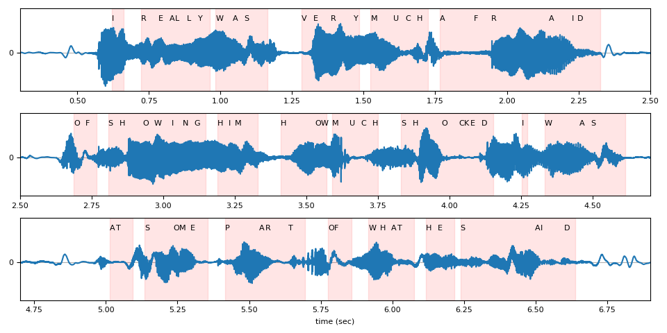
时步对齐
回想一下,结果假设的组件之一是与标记 ID 对应的时步。
timesteps = beam_search_result[0][0].timesteps
predicted_tokens = beam_search_decoder.idxs_to_tokens(beam_search_result[0][0].tokens)

print(predicted_tokens, len(predicted_tokens))
print(timesteps, timesteps.shape[0])
['|', 'i', '|', 'r', 'e', 'a', 'l', 'l', 'y', '|', 'w', 'a', 's', '|', 'v', 'e', 'r', 'y', '|', 'm', 'u', 'c', 'h', '|', 'a', 'f', 'r', 'a', 'i', 'd', '|', 'o', 'f', '|', 's', 'h', 'o', 'w', 'i', 'n', 'g', '|', 'h', 'i', 'm', '|', 'h', 'o', 'w', '|', 'm', 'u', 'c', 'h', '|', 's', 'h', 'o', 'c', 'k', 'e', 'd', '|', 'i', '|', 'w', 'a', 's', '|', 'a', 't', '|', 's', 'o', 'm', 'e', '|', 'p', 'a', 'r', 't', '|', 'o', 'f', '|', 'w', 'h', 'a', 't', '|', 'h', 'e', '|', 's', 'a', 'i', 'd', '|', '|'] 99
tensor([  0,  31,  33,  36,  39,  41,  42,  44,  46,  48,  49,  52,  54,  58,
         64,  66,  69,  73,  74,  76,  80,  82,  84,  86,  88,  94,  97, 107,
        111, 112, 116, 134, 136, 138, 140, 142, 146, 148, 151, 153, 155, 157,
        159, 161, 162, 166, 170, 176, 177, 178, 179, 182, 184, 186, 187, 191,
        193, 198, 201, 202, 203, 205, 207, 212, 213, 216, 222, 224, 230, 250,
        251, 254, 256, 261, 262, 264, 267, 270, 276, 277, 281, 284, 288, 289,
        292, 295, 297, 299, 300, 303, 305, 307, 310, 311, 324, 325, 329, 331,
        353], dtype=torch.int32) 99
下面,我们可视化了相对于原始波形的标记时步对齐。
def plot_alignments(waveform, emission, tokens, timesteps, sample_rate):

    t = torch.arange(waveform.size(0)) / sample_rate
    ratio = waveform.size(0) / emission.size(1) / sample_rate

    chars = []
    words = []
    word_start = None
    for token, timestep in zip(tokens, timesteps * ratio):
        if token == "|":
            if word_start is not None:
                words.append((word_start, timestep))
            word_start = None
        else:
            chars.append((token, timestep))
            if word_start is None:
                word_start = timestep

    fig, axes = plt.subplots(3, 1)

    def _plot(ax, xlim):
        ax.plot(t, waveform)
        for token, timestep in chars:
            ax.annotate(token.upper(), (timestep, 0.5))
        for word_start, word_end in words:
            ax.axvspan(word_start, word_end, alpha=0.1, color="red")
        ax.set_ylim(-0.6, 0.7)
        ax.set_yticks([0])
        ax.grid(True, axis="y")
        ax.set_xlim(xlim)

    _plot(axes[0], (0.3, 2.5))
    _plot(axes[1], (2.5, 4.7))
    _plot(axes[2], (4.7, 6.9))
    axes[2].set_xlabel("time (sec)")
    fig.tight_layout()


plot_alignments(waveform[0], emission, predicted_tokens, timesteps, bundle.sample_rate)
束搜索解码器参数
在本节中,我们将更深入地了解一些不同的参数和权衡。有关可定制参数的完整列表,请参阅 documentation。
辅助函数
def print_decoded(decoder, emission, param, param_value):
    start_time = time.monotonic()
    result = decoder(emission)
    decode_time = time.monotonic() - start_time

    transcript = " ".join(result[0][0].words).lower().strip()
    score = result[0][0].score
    print(f"{param} {param_value:<3}: {transcript} (score: {score:.2f}; {decode_time:.4f} secs)")
nbest
此参数指示要返回的最佳假设数,这是贪婪解码器无法实现的属性。例如,通过在前面构建束搜索解码器时将 nbest=3 设置,我们现在可以访问具有前 3 个分数的假设。
for i in range(3):
    transcript = " ".join(beam_search_result[0][i].words).strip()
    score = beam_search_result[0][i].score
    print(f"{transcript} (score: {score})")
i really was very much afraid of showing him how much shocked i was at some part of what he said (score: 3699.824109642502)
i really was very much afraid of showing him how much shocked i was at some parts of what he said (score: 3697.858373688456)
i reply was very much afraid of showing him how much shocked i was at some part of what he said (score: 3695.0157600045172)
束大小
beam_size 参数决定在每个解码步骤后保存的最大最佳假设数。使用更大的束大小允许探索更广泛的可能假设,这可以产生得分更高的假设,但计算成本更高,并且在超过一定点后不会提供额外增益。
在以下示例中,我们看到解码质量随着我们将束大小从 1 增加到 5 再到 50 而得到改进,但请注意,使用 500 的束大小与 50 的束大小提供了相同的输出,而增加了计算时间。
beam_sizes = [1, 5, 50, 500]

for beam_size in beam_sizes:
    beam_search_decoder = ctc_decoder(
        lexicon=files.lexicon,
        tokens=files.tokens,
        lm=files.lm,
        beam_size=beam_size,
        lm_weight=LM_WEIGHT,
        word_score=WORD_SCORE,
    )

    print_decoded(beam_search_decoder, emission, "beam size", beam_size)
beam size 1  : i you ery much afra of shongut shot i was at some arte what he sad (score: 3144.93; 0.0449 secs)
beam size 5  : i rely was very much afraid of showing him how much shot i was at some parts of what he said (score: 3688.02; 0.0516 secs)
beam size 50 : i really was very much afraid of showing him how much shocked i was at some part of what he said (score: 3699.82; 0.1667 secs)
beam size 500: i really was very much afraid of showing him how much shocked i was at some part of what he said (score: 3699.82; 0.5421 secs)
束大小标记
beam_size_token 参数对应于在解码步骤中为每个假设扩展而要考虑的标记数。探索更多可能的下一个标记会增加潜在假设的范围,但会以计算为代价。
num_tokens = len(tokens)
beam_size_tokens = [1, 5, 10, num_tokens]

for beam_size_token in beam_size_tokens:
    beam_search_decoder = ctc_decoder(
        lexicon=files.lexicon,
        tokens=files.tokens,
        lm=files.lm,
        beam_size_token=beam_size_token,
        lm_weight=LM_WEIGHT,
        word_score=WORD_SCORE,
    )

    print_decoded(beam_search_decoder, emission, "beam size token", beam_size_token)
beam size token 1  : i rely was very much affray of showing him hoch shot i was at some part of what he sed (score: 3584.80; 0.1642 secs)
beam size token 5  : i rely was very much afraid of showing him how much shocked i was at some part of what he said (score: 3694.83; 0.1812 secs)
beam size token 10 : i really was very much afraid of showing him how much shocked i was at some part of what he said (score: 3696.25; 0.2047 secs)
beam size token 29 : i really was very much afraid of showing him how much shocked i was at some part of what he said (score: 3699.82; 0.2323 secs)
束阈值
beam_threshold 参数用于在每个解码步骤中修剪存储的假设集,删除得分比最高得分假设高出 beam_threshold 的假设。在选择较小的阈值以修剪更多假设并减少搜索空间,以及选择足够大的阈值以避免修剪合理假设之间存在平衡。
beam_thresholds = [1, 5, 10, 25]

for beam_threshold in beam_thresholds:
    beam_search_decoder = ctc_decoder(
        lexicon=files.lexicon,
        tokens=files.tokens,
        lm=files.lm,
        beam_threshold=beam_threshold,
        lm_weight=LM_WEIGHT,
        word_score=WORD_SCORE,
    )

    print_decoded(beam_search_decoder, emission, "beam threshold", beam_threshold)
beam threshold 1  : i ila ery much afraid of shongut shot i was at some parts of what he said (score: 3316.20; 0.0282 secs)
beam threshold 5  : i rely was very much afraid of showing him how much shot i was at some parts of what he said (score: 3682.23; 0.0696 secs)
beam threshold 10 : i really was very much afraid of showing him how much shocked i was at some part of what he said (score: 3699.82; 0.2163 secs)
beam threshold 25 : i really was very much afraid of showing him how much shocked i was at some part of what he said (score: 3699.82; 0.2386 secs)
语言模型权重
lm_weight 参数是分配给语言模型分数的权重,该分数将与声学模型分数累加,以确定总分。更大的权重鼓励模型根据语言模型预测下一个词,而更小的权重则更重视声学模型分数。
lm_weights = [0, LM_WEIGHT, 15]

for lm_weight in lm_weights:
    beam_search_decoder = ctc_decoder(
        lexicon=files.lexicon,
        tokens=files.tokens,
        lm=files.lm,
        lm_weight=lm_weight,
        word_score=WORD_SCORE,
    )

    print_decoded(beam_search_decoder, emission, "lm weight", lm_weight)
lm weight 0  : i rely was very much affraid of showing him ho much shoke i was at some parte of what he seid (score: 3834.05; 0.2603 secs)
lm weight 3.23: i really was very much afraid of showing him how much shocked i was at some part of what he said (score: 3699.82; 0.2660 secs)
lm weight 15 : was there in his was at some of what he said (score: 2918.99; 0.2454 secs)
其他参数
可以优化的其他参数包括以下内容
word_score:单词结束时要添加的分数unk_score:要添加的未知单词出现分数sil_score:要添加的静音出现分数log_add:是否对词典 Trie 扩散使用对数加法
脚本的总运行时间:(2 分 51.705 秒)
