在上一篇文章中,我们回顾了自动微分的理论基础,并探讨了 PyTorch 中的实现。在本文中,我们将展示 PyTorch 中涉及创建和执行计算图的部分。为了理解以下内容,请阅读 @ezyang 关于 PyTorch 内部原理的精彩博客文章。
Autograd 组件
首先,让我们看看 Autograd 的不同组件所在的位置。
tools/autograd:在这里我们可以找到导数的定义,正如我们在上一篇文章中看到的derivatives.yaml,以及几个 Python 脚本和一个名为templates的文件夹。这些脚本和模板在构建时用于根据 yaml 文件中指定的导数生成 C++ 代码。此外,这里的脚本还为常规的 ATen 函数生成包装器,以便构建计算图。
torch/autograd:这个文件夹存放着可以直接从 Python 使用的 Autograd 组件。在function.py中,我们找到了torch.autograd.Function的实际定义,这是一个供用户根据文档在 Python 中编写自己的可微分函数时使用的类。functional.py包含用于函数式计算给定函数的雅可比向量积、Hessian 和其他梯度相关计算的组件。其余文件包含其他组件,例如梯度检查器、异常检测和 Autograd 分析器。
torch/csrc/autograd:这里是图创建和执行相关代码的所在地。所有这些代码都用 C++ 编写,因为它是一个要求极高性能的关键部分。在这里,我们有几个文件实现了引擎、元数据存储和所有必需的组件。此外,我们还有几个文件以python_开头,它们的主要职责是允许在 Autograd 引擎中使用 Python 对象。
图的创建
此前,我们描述了计算图的创建。现在,我们将通过引用实际代码库来了解 PyTorch 如何创建这些图。
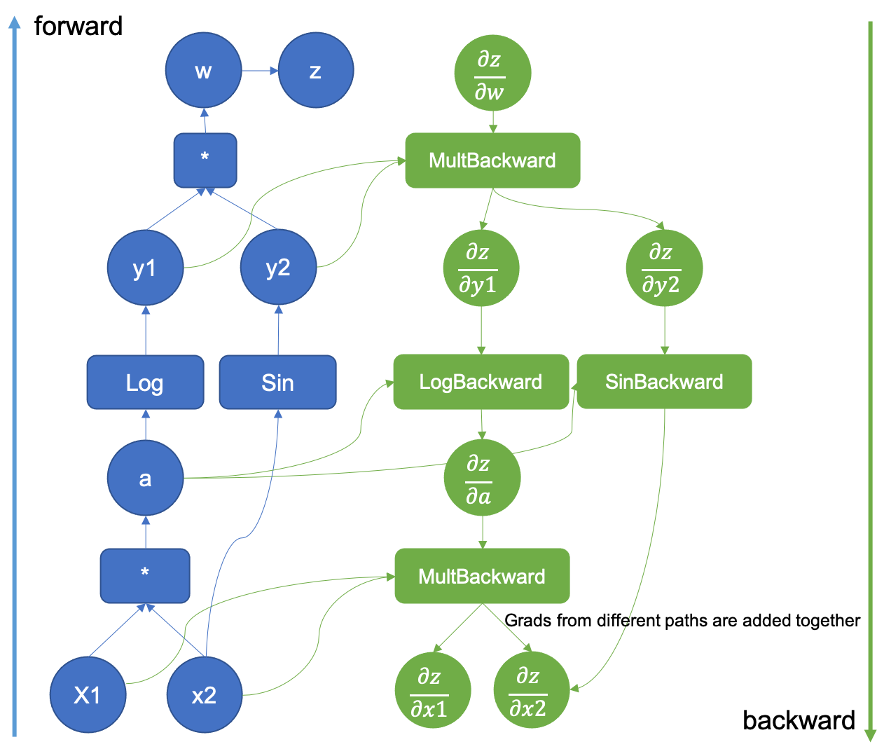
图 1:增强型计算图示例
这一切都始于我们的 Python 代码中,当我们请求一个张量需要梯度时。
>>> x = torch.tensor([0.5, 0.75], requires_grad=True)
在张量创建时设置required_grad标志后,c10 将分配一个AutogradMeta对象,该对象用于保存图信息。
void TensorImpl::set_requires_grad(bool requires_grad) {
  ...
  if (!autograd_meta_)
    autograd_meta_ = impl::GetAutogradMetaFactory()->make();
    autograd_meta_->set_requires_grad(requires_grad, this);
}
AutogradMeta对象在torch/csrc/autograd/variable.h中定义如下:
struct TORCH_API AutogradMeta : public c10::AutogradMetaInterface {
  std::string name_;

  Variable grad_;
  std::shared_ptr<Node> grad_fn_;
  std::weak_ptr<Node> grad_accumulator_;
  // other fields and methods
  ...
};
此结构中最重要的字段是grad_中计算的梯度以及指向函数grad_fn的指针,该函数将由引擎调用以生成实际梯度。此外,还有一个梯度累加器对象,用于将此张量所涉及的所有不同梯度相加,我们将在图执行中看到。
图、节点和边。
现在,当我们调用一个以该张量为参数的可微分函数时,相关的元数据将被填充。假设我们调用一个在 ATen 中实现的常规 torch 函数。例如,像我们之前的博客文章示例中的乘法。生成的张量有一个名为grad_fn的字段,它本质上是指向用于计算该操作梯度的函数的指针。
>>> x = torch.tensor([0.5, 0.75], requires_grad=True)
>>> v = x[0] * x[1]
>>> v
tensor(0.3750, grad_fn=<MulBackward0>)
在这里,我们看到张量的grad_fn具有MulBackward0值。此函数与derivatives.yaml文件中的函数相同,其 C++ 代码由tools/autograd中的所有脚本自动生成。其自动生成的源代码可以在torch/csrc/autograd/generated/Functions.cpp中看到。
variable_list MulBackward0::apply(variable_list&& grads) {
  std::lock_guard<std::mutex> lock(mutex_);

  IndexRangeGenerator gen;
  auto self_ix = gen.range(1);
  auto other_ix = gen.range(1);
  variable_list grad_inputs(gen.size());
  auto& grad = grads[0];
  auto self = self_.unpack();
  auto other = other_.unpack();
  bool any_grad_defined = any_variable_defined(grads);
  if (should_compute_output({ other_ix })) {
    auto grad_result = any_grad_defined ? (mul_tensor_backward(grad, self, other_scalar_type)) : Tensor();
    copy_range(grad_inputs, other_ix, grad_result);
  }
  if (should_compute_output({ self_ix })) {
    auto grad_result = any_grad_defined ? (mul_tensor_backward(grad, other, self_scalar_type)) : Tensor();
    copy_range(grad_inputs, self_ix, grad_result);
  }
  return grad_inputs;
}
grad_fn对象继承自TraceableFunction类,它是Node的子类,仅设置了一个属性以启用用于调试和优化的跟踪。根据定义,图具有节点和边,因此这些函数确实是计算图的节点,它们通过使用Edge对象连接在一起,以便稍后进行图遍历。
Node的定义可以在torch/csrc/autograd/function.h文件中找到。
struct TORCH_API Node : std::enable_shared_from_this<Node> {
 ...
 /// Evaluates the function on the given inputs and returns the result of the
  /// function call.
  variable_list operator()(variable_list&& inputs) {
  ...
  }

protected:
  /// Performs the `Node`'s actual operation.
  virtual variable_list apply(variable_list&& inputs) = 0;
  …
  edge_list next_edges_;
本质上,我们看到它重写了执行实际函数调用的operator (),以及一个纯虚函数apply。正如我们在上面的MulBackward0示例中看到的那样,自动生成的函数会重写此apply方法。最后,节点还包含一个边列表,以实现图连接。
Edge对象用于将Node连接在一起,其实现非常简单。
struct Edge {
  ...
  /// The function this `Edge` points to.
  std::shared_ptr<Node> function;
  /// The identifier of a particular input to the function.
  uint32_t input_nr;
};
它只需要一个函数指针(边连接在一起的实际grad_fn对象)和一个用作边 ID 的输入编号。
连接节点
当我们调用两个张量的乘法运算时,我们进入了自动生成代码的领域。我们在tools/autograd中看到的所有脚本都填充了一系列模板,这些模板封装了 ATen 中的可微分函数。这些函数包含在正向传播期间构建反向图的代码。
gen_variable_type.py脚本负责编写所有这些包装代码。这个脚本在 PyTorch 构建过程中从tools/autograd/gen_autograd.py调用,它将自动生成的函数包装器输出到torch/csrc/autograd/generated/。
让我们看看张量乘法生成的函数是什么样子的。代码已经简化,但在从源代码编译 PyTorch 时可以在torch/csrc/autograd/generated/VariableType_4.cpp文件中找到它。
at::Tensor mul_Tensor(c10::DispatchKeySet ks, const at::Tensor & self, const at::Tensor & other) {
  ...
  auto _any_requires_grad = compute_requires_grad( self, other );
  std::shared_ptr<MulBackward0> grad_fn;
  if (_any_requires_grad) {
    // Creates the link to the actual grad_fn and links the graph for backward traversal
    grad_fn = std::shared_ptr<MulBackward0>(new MulBackward0(), deleteNode);
    grad_fn->set_next_edges(collect_next_edges( self, other ));
    ...
  }
  …
  // Does the actual function call to ATen
  auto _tmp = ([&]() {
    at::AutoDispatchBelowADInplaceOrView guard;
    return at::redispatch::mul(ks & c10::after_autograd_keyset, self_, other_);
  })();

  auto result = std::move(_tmp);
    if (grad_fn) {
       // Connects the result to the graph
      set_history(flatten_tensor_args( result ), grad_fn);
  }
  ...
  return result;
}
让我们仔细研究一下这段代码中最重要的几行。首先,grad_fn对象是使用:` grad_fn = std::shared_ptr(new MulBackward0(), deleteNode);`创建的。
在创建grad_fn对象之后,用于连接节点的边是使用grad_fn->set_next_edges(collect_next_edges( self, other ));调用创建的。
struct MakeNextFunctionList : IterArgs<MakeNextFunctionList> {
  edge_list next_edges;
  using IterArgs<MakeNextFunctionList>::operator();
  void operator()(const Variable& variable) {
    if (variable.defined()) {
      next_edges.push_back(impl::gradient_edge(variable));
    } else {
      next_edges.emplace_back();
    }
  }
  void operator()(const c10::optional<Variable>& variable) {
    if (variable.has_value() && variable->defined()) {
      next_edges.push_back(impl::gradient_edge(*variable));
    } else {
      next_edges.emplace_back();
    }
  }
};

template <typename... Variables>
edge_list collect_next_edges(Variables&&... variables) {
  detail::MakeNextFunctionList make;
  make.apply(std::forward<Variables>(variables)...);
  return std::move(make.next_edges);
}
给定一个输入变量(它只是一个常规张量),collect_next_edges将通过调用impl::gradient_edge来创建一个Edge对象。
 Edge gradient_edge(const Variable& self) {
    // If grad_fn is null (as is the case for a leaf node), we instead
    // interpret the gradient function to be a gradient accumulator, which will
    // accumulate its inputs into the grad property of the variable. These
    // nodes get suppressed in some situations, see "suppress gradient
    // accumulation" below. Note that only variables which have `requires_grad =
    // True` can have gradient accumulators.
    if (const auto& gradient = self.grad_fn()) {
      return Edge(gradient, self.output_nr());
    } else {
      return Edge(grad_accumulator(self), 0);
    }
  }
要理解边的工作原理,假设一个早期执行的函数产生了两个输出张量,两者都设置了它们的grad_fn,每个张量还有一个output_nr属性,表示它们返回的顺序。当为当前的grad_fn创建边时,每个输入变量都会创建一个Edge对象。这些边将指向变量的grad_fn,并且还将跟踪output_nr以建立在遍历图时使用的ID。如果输入变量是“叶子”(即它们不是由任何可微分函数产生的),则它们没有设置grad_fn属性。默认情况下会设置一个名为梯度累加器的特殊函数,如上面的代码片段所示。
边创建完成后,当前正在创建的grad_fn图节点对象将使用set_next_edges函数来保存它们。这就是将grad_fn连接在一起,从而生成计算图的过程。
 void set_next_edges(edge_list&& next_edges) {
    next_edges_ = std::move(next_edges);
    for(const auto& next_edge : next_edges_) {
      update_topological_nr(next_edge);
    }
  }
现在,函数的前向传播将执行,执行后set_history会将输出张量连接到grad_fn节点。
inline void set_history(
    at::Tensor& variable,
    const std::shared_ptr<Node>& grad_fn) {
  AT_ASSERT(grad_fn);
  if (variable.defined()) {
    // If the codegen triggers this, you most likely want to add your newly added function
    // to the DONT_REQUIRE_DERIVATIVE list in tools/autograd/gen_variable_type.py
    TORCH_INTERNAL_ASSERT(isDifferentiableType(variable.scalar_type()));
    auto output_nr =
        grad_fn->add_input_metadata(variable);
    impl::set_gradient_edge(variable, {grad_fn, output_nr});
  } else {
    grad_fn->add_input_metadata(Node::undefined_input());
  }
}
set_history调用set_gradient_edge,它只是将 grad_fn 和output_nr复制到张量拥有的AutogradMeta对象中。
 void set_gradient_edge(const Variable& self, Edge edge) {
    auto* meta = materialize_autograd_meta(self);
    meta->grad_fn_ = std::move(edge.function);
    meta->output_nr_ = edge.input_nr;
    // For views, make sure this new grad_fn_ is not overwritten unless it is necessary
    // in the VariableHooks::grad_fn below.
    // This logic is only relevant for custom autograd Functions for which multiple
    // operations can happen on a given Tensor before its gradient edge is set when
    // exiting the custom Function.
    auto diff_view_meta = get_view_autograd_meta(self);
    if (diff_view_meta && diff_view_meta->has_bw_view()) {
      diff_view_meta->set_attr_version(self._version());
    }
  }
现在,这个张量将作为另一个函数的输入,并且上述所有步骤都将重复。请查看下面的动画,了解图是如何创建的。
图 2:显示图创建的动画
在图中注册 Python 函数
我们已经了解了 Autograd 如何为 ATen 中包含的函数创建图。然而,当我们用 Python 定义可微分函数时,它们也包含在图中!
一个 Autograd Python 定义的函数如下所示:
class Exp(torch.autograd.Function):
     @staticmethod
     def forward(ctx, i):
         result = i.exp()
         ctx.save_for_backward(result)
         return result

     @staticmethod
     def backward(ctx, grad_output):
         result, = ctx.saved_tensors
         return grad_output * result

# Call the function
Exp.apply(torch.tensor(0.5, requires_grad=True))
# Outputs: tensor(1.6487, grad_fn=<ExpBackward>)
在上面的代码片段中,Autograd 在创建图时检测到我们的 Python 函数。所有这一切都归功于Function类。让我们看看当我们调用apply时会发生什么。
apply在torch._C._FunctionBase类中定义,但此类不存在于 Python 源代码中。_FunctionBase是使用 Python C API 将 C 函数连接到单个 Python 类中,从而在 C++ 中定义的。我们正在寻找一个名为THPFunction_apply的函数。
PyObject *THPFunction_apply(PyObject *cls, PyObject *inputs)
{

  // Generates the graph node
  THPObjectPtr backward_cls(PyObject_GetAttrString(cls, "_backward_cls"));
  if (!backward_cls) return nullptr;
  THPObjectPtr ctx_obj(PyObject_CallFunctionObjArgs(backward_cls, nullptr));
  if (!ctx_obj) return nullptr;
  THPFunction* ctx = (THPFunction*)ctx_obj.get();

  auto cdata = std::shared_ptr<PyNode>(new PyNode(std::move(ctx_obj)), deleteNode);
  ctx->cdata = cdata;

  // Prepare inputs and allocate context (grad fn)
  // Unpack inputs will collect the edges
  auto info_pair = unpack_input<false>(inputs);
  UnpackedInput& unpacked_input = info_pair.first;
  InputFlags& input_info = info_pair.second;

   // Initialize backward function (and ctx)
  bool is_executable = input_info.is_executable;
  cdata->set_next_edges(std::move(input_info.next_edges));
  ctx->needs_input_grad = input_info.needs_input_grad.release();
  ctx->is_variable_input = std::move(input_info.is_variable_input);

  // Prepend ctx to input_tuple, in preparation for static method call
  auto num_args = PyTuple_GET_SIZE(inputs);
  THPObjectPtr ctx_input_tuple(PyTuple_New(num_args + 1));
  if (!ctx_input_tuple) return nullptr;
  Py_INCREF(ctx);
  PyTuple_SET_ITEM(ctx_input_tuple.get(), 0, (PyObject*)ctx);
  for (int i = 0; i < num_args; ++i) {
    PyObject *arg = PyTuple_GET_ITEM(unpacked_input.input_tuple.get(), i);
    Py_INCREF(arg);
    PyTuple_SET_ITEM(ctx_input_tuple.get(), i + 1, arg);
  }

  // Call forward
  THPObjectPtr tensor_outputs;
  {
    AutoGradMode grad_mode(false);
    THPObjectPtr forward_fn(PyObject_GetAttrString(cls, "forward"));
    if (!forward_fn) return nullptr;
    tensor_outputs = PyObject_CallObject(forward_fn, ctx_input_tuple);
    if (!tensor_outputs) return nullptr;
  }

  // Here is where the outputs gets the tensors tracked
  return process_outputs(cls, cdata, ctx, unpacked_input, inputs, std::move(tensor_outputs),
                         is_executable, node);
  END_HANDLE_TH_ERRORS
}
尽管由于所有的 Python API 调用,这段代码一开始难以阅读,但它本质上与我们为 ATen 看到的自动生成的前向函数做着相同的事情。
创建grad_fn对象。收集边以将当前的grad_fn与输入张量链接起来。执行函数forward。将创建的grad_fn分配给输出张量元数据。
grad_fn对象是在以下位置创建的:
  // Generates the graph node
  THPObjectPtr backward_cls(PyObject_GetAttrString(cls, "_backward_cls"));
  if (!backward_cls) return nullptr;
  THPObjectPtr ctx_obj(PyObject_CallFunctionObjArgs(backward_cls, nullptr));
  if (!ctx_obj) return nullptr;
  THPFunction* ctx = (THPFunction*)ctx_obj.get();

  auto cdata = std::shared_ptr<PyNode>(new PyNode(std::move(ctx_obj)), deleteNode);
  ctx->cdata = cdata;
基本上,它要求 Python API 获取指向可以执行用户编写函数的 Python 对象的指针。然后,它将其包装到一个PyNode对象中,这是一个专门的Node对象,当在正向传播期间执行apply时,它会使用提供的 Python 函数调用 Python 解释器。请注意,在代码中,cdata是图的一部分的实际Node对象。ctx是传递给 Python forward/backward函数的对象,用户函数和 PyTorch 都使用它来存储自动梯度相关信息。
与常规 C++ 函数一样,我们也调用collect_next_edges来跟踪输入的grad_fn对象,但这在unpack_input中完成。
template<bool enforce_variables>
std::pair<UnpackedInput, InputFlags> unpack_input(PyObject *args) {
  ...
  flags.next_edges = (flags.is_executable ? collect_next_edges(unpacked.input_vars) : edge_list());
  return std::make_pair(std::move(unpacked), std::move(flags));
}
之后,通过执行cdata->set_next_edges(std::move(input_info.next_edges));将边分配给grad_fn,并通过 Python 解释器 C API 调用前向函数。
一旦输出张量从前向传播返回,它们将在process_outputs函数中进行处理并转换为变量。
PyObject* process_outputs(PyObject *op_obj, const std::shared_ptr<PyNode>& cdata,
                          THPFunction* grad_fn, const UnpackedInput& unpacked,
                          PyObject *inputs, THPObjectPtr&& raw_output, bool is_executable,
                          torch::jit::Node* node) {
  ...
  _wrap_outputs(cdata, grad_fn, unpacked.input_vars, raw_output, outputs, is_executable);
  _trace_post_record(node, op_obj, unpacked.input_vars, outputs, is_inplace, unpack_output);
  if (is_executable) {
    _save_variables(cdata, grad_fn);
  } ...
  return outputs.release();
}
在这里,_wrap_outputs负责将前向输出的grad_fn设置为新创建的那个。为此,它调用了另一个在不同文件中定义的_wrap_outputs函数,所以这里的过程有点令人困惑。
static void _wrap_outputs(const std::shared_ptr<PyNode>& cdata, THPFunction *self,
    const variable_list &input_vars, PyObject *raw_output, PyObject *outputs, bool is_executable)
{
  auto cdata_if_executable = is_executable ? cdata : nullptr;
 ...

  // Wrap only the tensor outputs.
  // This calls csrc/autograd/custom_function.cpp
  auto wrapped_outputs = _wrap_outputs(input_vars, non_differentiable, dirty_inputs, raw_output_vars, cdata_if_executable);
...
}
被调用的_wrap_outputs负责在输出张量中设置 autograd 元数据。
std::vector<c10::optional<Variable>> _wrap_outputs(const variable_list &input_vars,
  const std::unordered_set<at::TensorImpl*> &non_differentiable,
  const std::unordered_set<at::TensorImpl*> &dirty_inputs,
  const at::ArrayRef<c10::optional<Variable>> raw_outputs,
  const std::shared_ptr<Node> &cdata) {


  std::unordered_set<at::TensorImpl*> inputs;
  …
  // Sets the grad_fn and output_nr of an output Variable.
  auto set_history = [&](Variable& var, uint32_t output_nr, bool is_input, bool is_modified,
                         bool is_differentiable) {
    // Lots of checks
    if (!is_differentiable) {
     ...
    } else if (is_input) {
      // An input has been returned, but it wasn't modified. Return it as a view
      // so that we can attach a new grad_fn to the Variable.
      // Run in no_grad mode to mimic the behavior of the forward.
      {
        AutoGradMode grad_mode(false);
        var = var.view_as(var);
      }
      impl::set_gradient_edge(var, {cdata, output_nr});
    } else if (cdata) {
      impl::set_gradient_edge(var, {cdata, output_nr});
    }
  };
这就是调用set_gradient_edge的地方,也是用户编写的 Python 函数如何通过其关联的反向函数包含在计算图中的方式!
结束语
这篇博客文章旨在概述 PyTorch 如何构建我们在上一篇文章中讨论的实际计算图。下一篇将讨论 Autograd 引擎如何执行这些图。